- Alternatives

10 Methods of Data Presentation That Really Work in 2024
Leah Nguyen • 20 August, 2024 • 13 min read
Have you ever presented a data report to your boss/coworkers/teachers thinking it was super dope like you’re some cyber hacker living in the Matrix, but all they saw was a pile of static numbers that seemed pointless and didn't make sense to them?
Understanding digits is rigid . Making people from non-analytical backgrounds understand those digits is even more challenging.
How can you clear up those confusing numbers and make your presentation as clear as the day? Let's check out these best ways to present data. 💎
| How many type of charts are available to present data? | 7 |
| How many charts are there in statistics? | 4, including bar, line, histogram and pie. |
| How many types of charts are available in Excel? | 8 |
| Who invented charts? | William Playfair |
| When were the charts invented? | 18th Century |
More Tips with AhaSlides
- Marketing Presentation
- Survey Result Presentation
- Types of Presentation

Start in seconds.
Get any of the above examples as templates. Sign up for free and take what you want from the template library!
Data Presentation - What Is It?
The term ’data presentation’ relates to the way you present data in a way that makes even the most clueless person in the room understand.
Some say it’s witchcraft (you’re manipulating the numbers in some ways), but we’ll just say it’s the power of turning dry, hard numbers or digits into a visual showcase that is easy for people to digest.
Presenting data correctly can help your audience understand complicated processes, identify trends, and instantly pinpoint whatever is going on without exhausting their brains.
Good data presentation helps…
- Make informed decisions and arrive at positive outcomes . If you see the sales of your product steadily increase throughout the years, it’s best to keep milking it or start turning it into a bunch of spin-offs (shoutout to Star Wars👀).
- Reduce the time spent processing data . Humans can digest information graphically 60,000 times faster than in the form of text. Grant them the power of skimming through a decade of data in minutes with some extra spicy graphs and charts.
- Communicate the results clearly . Data does not lie. They’re based on factual evidence and therefore if anyone keeps whining that you might be wrong, slap them with some hard data to keep their mouths shut.
- Add to or expand the current research . You can see what areas need improvement, as well as what details often go unnoticed while surfing through those little lines, dots or icons that appear on the data board.
Methods of Data Presentation and Examples
Imagine you have a delicious pepperoni, extra-cheese pizza. You can decide to cut it into the classic 8 triangle slices, the party style 12 square slices, or get creative and abstract on those slices.
There are various ways to cut a pizza and you get the same variety with how you present your data. In this section, we will bring you the 10 ways to slice a pizza - we mean to present your data - that will make your company’s most important asset as clear as day. Let's dive into 10 ways to present data efficiently.
#1 - Tabular
Among various types of data presentation, tabular is the most fundamental method, with data presented in rows and columns. Excel or Google Sheets would qualify for the job. Nothing fancy.

This is an example of a tabular presentation of data on Google Sheets. Each row and column has an attribute (year, region, revenue, etc.), and you can do a custom format to see the change in revenue throughout the year.
When presenting data as text, all you do is write your findings down in paragraphs and bullet points, and that’s it. A piece of cake to you, a tough nut to crack for whoever has to go through all of the reading to get to the point.
- 65% of email users worldwide access their email via a mobile device.
- Emails that are optimised for mobile generate 15% higher click-through rates.
- 56% of brands using emojis in their email subject lines had a higher open rate.
(Source: CustomerThermometer )
All the above quotes present statistical information in textual form. Since not many people like going through a wall of texts, you’ll have to figure out another route when deciding to use this method, such as breaking the data down into short, clear statements, or even as catchy puns if you’ve got the time to think of them.
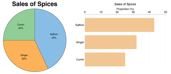
#3 - Pie chart
A pie chart (or a ‘donut chart’ if you stick a hole in the middle of it) is a circle divided into slices that show the relative sizes of data within a whole. If you’re using it to show percentages, make sure all the slices add up to 100%.

The pie chart is a familiar face at every party and is usually recognised by most people. However, one setback of using this method is our eyes sometimes can’t identify the differences in slices of a circle, and it’s nearly impossible to compare similar slices from two different pie charts, making them the villains in the eyes of data analysts.

#4 - Bar chart
The bar chart is a chart that presents a bunch of items from the same category, usually in the form of rectangular bars that are placed at an equal distance from each other. Their heights or lengths depict the values they represent.
They can be as simple as this:

Or more complex and detailed like this example of data presentation. Contributing to an effective statistic presentation, this one is a grouped bar chart that not only allows you to compare categories but also the groups within them as well.

#5 - Histogram
Similar in appearance to the bar chart but the rectangular bars in histograms don’t often have the gap like their counterparts.
Instead of measuring categories like weather preferences or favourite films as a bar chart does, a histogram only measures things that can be put into numbers.

Teachers can use presentation graphs like a histogram to see which score group most of the students fall into, like in this example above.
#6 - Line graph
Recordings to ways of displaying data, we shouldn't overlook the effectiveness of line graphs. Line graphs are represented by a group of data points joined together by a straight line. There can be one or more lines to compare how several related things change over time.

On a line chart’s horizontal axis, you usually have text labels, dates or years, while the vertical axis usually represents the quantity (e.g.: budget, temperature or percentage).
#7 - Pictogram graph
A pictogram graph uses pictures or icons relating to the main topic to visualise a small dataset. The fun combination of colours and illustrations makes it a frequent use at schools.
Pictograms are a breath of fresh air if you want to stay away from the monotonous line chart or bar chart for a while. However, they can present a very limited amount of data and sometimes they are only there for displays and do not represent real statistics.
#8 - Radar chart
If presenting five or more variables in the form of a bar chart is too stuffy then you should try using a radar chart, which is one of the most creative ways to present data.
Radar charts show data in terms of how they compare to each other starting from the same point. Some also call them ‘spider charts’ because each aspect combined looks like a spider web.

Radar charts can be a great use for parents who’d like to compare their child’s grades with their peers to lower their self-esteem. You can see that each angular represents a subject with a score value ranging from 0 to 100. Each student’s score across 5 subjects is highlighted in a different colour.

If you think that this method of data presentation somehow feels familiar, then you’ve probably encountered one while playing Pokémon .
#9 - Heat map
A heat map represents data density in colours. The bigger the number, the more colour intensity that data will be represented.

Most US citizens would be familiar with this data presentation method in geography. For elections, many news outlets assign a specific colour code to a state, with blue representing one candidate and red representing the other. The shade of either blue or red in each state shows the strength of the overall vote in that state.

Another great thing you can use a heat map for is to map what visitors to your site click on. The more a particular section is clicked the ‘hotter’ the colour will turn, from blue to bright yellow to red.
#10 - Scatter plot
If you present your data in dots instead of chunky bars, you’ll have a scatter plot.
A scatter plot is a grid with several inputs showing the relationship between two variables. It’s good at collecting seemingly random data and revealing some telling trends.

For example, in this graph, each dot shows the average daily temperature versus the number of beach visitors across several days. You can see that the dots get higher as the temperature increases, so it’s likely that hotter weather leads to more visitors.
5 Data Presentation Mistakes to Avoid
#1 - assume your audience understands what the numbers represent.
You may know all the behind-the-scenes of your data since you’ve worked with them for weeks, but your audience doesn’t.

Showing without telling only invites more and more questions from your audience, as they have to constantly make sense of your data, wasting the time of both sides as a result.
While showing your data presentations, you should tell them what the data are about before hitting them with waves of numbers first. You can use interactive activities such as polls , word clouds , online quizzes and Q&A sections , combined with icebreaker games , to assess their understanding of the data and address any confusion beforehand.
#2 - Use the wrong type of chart
Charts such as pie charts must have a total of 100% so if your numbers accumulate to 193% like this example below, you’re definitely doing it wrong.

Before making a chart, ask yourself: what do I want to accomplish with my data? Do you want to see the relationship between the data sets, show the up and down trends of your data, or see how segments of one thing make up a whole?
Remember, clarity always comes first. Some data visualisations may look cool, but if they don’t fit your data, steer clear of them.
#3 - Make it 3D
3D is a fascinating graphical presentation example. The third dimension is cool, but full of risks.
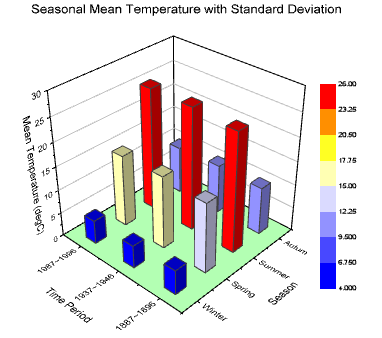
Can you see what’s behind those red bars? Because we can’t either. You may think that 3D charts add more depth to the design, but they can create false perceptions as our eyes see 3D objects closer and bigger than they appear, not to mention they cannot be seen from multiple angles.
#4 - Use different types of charts to compare contents in the same category
This is like comparing a fish to a monkey. Your audience won’t be able to identify the differences and make an appropriate correlation between the two data sets.
Next time, stick to one type of data presentation only. Avoid the temptation of trying various data visualisation methods in one go and make your data as accessible as possible.
#5 - Bombard the audience with too much information
The goal of data presentation is to make complex topics much easier to understand, and if you’re bringing too much information to the table, you’re missing the point.

The more information you give, the more time it will take for your audience to process it all. If you want to make your data understandable and give your audience a chance to remember it, keep the information within it to an absolute minimum. You should end your session with open-ended questions to see what your participants really think.
What are the Best Methods of Data Presentation?
Finally, which is the best way to present data?
The answer is…
There is none! Each type of presentation has its own strengths and weaknesses and the one you choose greatly depends on what you’re trying to do.
For example:
- Go for a scatter plot if you’re exploring the relationship between different data values, like seeing whether the sales of ice cream go up because of the temperature or because people are just getting more hungry and greedy each day?
- Go for a line graph if you want to mark a trend over time.
- Go for a heat map if you like some fancy visualisation of the changes in a geographical location, or to see your visitors' behaviour on your website.
- Go for a pie chart (especially in 3D) if you want to be shunned by others because it was never a good idea👇

Frequently Asked Questions
What is a chart presentation.
A chart presentation is a way of presenting data or information using visual aids such as charts, graphs, and diagrams. The purpose of a chart presentation is to make complex information more accessible and understandable for the audience.
When can I use charts for the presentation?
Charts can be used to compare data, show trends over time, highlight patterns, and simplify complex information.
Why should you use charts for presentation?
You should use charts to ensure your contents and visuals look clean, as they are the visual representative, provide clarity, simplicity, comparison, contrast and super time-saving!
What are the 4 graphical methods of presenting data?
Histogram, Smoothed frequency graph, Pie diagram or Pie chart, Cumulative or ogive frequency graph, and Frequency Polygon.

Leah Nguyen
Words that convert, stories that stick. I turn complex ideas into engaging narratives - helping audiences learn, remember, and take action.
Tips to Engage with Polls & Trivia
More from AhaSlides

Data presentation: A comprehensive guide
Learn how to create data presentation effectively and communicate your insights in a way that is clear, concise, and engaging.
Raja Bothra
Building presentations

Hey there, fellow data enthusiast!
Welcome to our comprehensive guide on data presentation.
Whether you're an experienced presenter or just starting, this guide will help you present your data like a pro. We'll dive deep into what data presentation is, why it's crucial, and how to master it. So, let's embark on this data-driven journey together.
What is data presentation?
Data presentation is the art of transforming raw data into a visual format that's easy to understand and interpret. It's like turning numbers and statistics into a captivating story that your audience can quickly grasp. When done right, data presentation can be a game-changer, enabling you to convey complex information effectively.
Why are data presentations important?
Imagine drowning in a sea of numbers and figures. That's how your audience might feel without proper data presentation. Here's why it's essential:
- Clarity : Data presentations make complex information clear and concise.
- Engagement : Visuals, such as charts and graphs, grab your audience's attention.
- Comprehension : Visual data is easier to understand than long, numerical reports.
- Decision-making : Well-presented data aids informed decision-making.
- Impact : It leaves a lasting impression on your audience.
Types of data presentation:
Now, let's delve into the diverse array of data presentation methods, each with its own unique strengths and applications. We have three primary types of data presentation, and within these categories, numerous specific visualization techniques can be employed to effectively convey your data.
1. Textual presentation
Textual presentation harnesses the power of words and sentences to elucidate and contextualize your data. This method is commonly used to provide a narrative framework for the data, offering explanations, insights, and the broader implications of your findings. It serves as a foundation for a deeper understanding of the data's significance.
2. Tabular presentation
Tabular presentation employs tables to arrange and structure your data systematically. These tables are invaluable for comparing various data groups or illustrating how data evolves over time. They present information in a neat and organized format, facilitating straightforward comparisons and reference points.
3. Graphical presentation
Graphical presentation harnesses the visual impact of charts and graphs to breathe life into your data. Charts and graphs are powerful tools for spotlighting trends, patterns, and relationships hidden within the data. Let's explore some common graphical presentation methods:
- Bar charts: They are ideal for comparing different categories of data. In this method, each category is represented by a distinct bar, and the height of the bar corresponds to the value it represents. Bar charts provide a clear and intuitive way to discern differences between categories.
- Pie charts: It excel at illustrating the relative proportions of different data categories. Each category is depicted as a slice of the pie, with the size of each slice corresponding to the percentage of the total value it represents. Pie charts are particularly effective for showcasing the distribution of data.
- Line graphs: They are the go-to choice when showcasing how data evolves over time. Each point on the line represents a specific value at a particular time period. This method enables viewers to track trends and fluctuations effortlessly, making it perfect for visualizing data with temporal dimensions.
- Scatter plots: They are the tool of choice when exploring the relationship between two variables. In this method, each point on the plot represents a pair of values for the two variables in question. Scatter plots help identify correlations, outliers, and patterns within data pairs.
The selection of the most suitable data presentation method hinges on the specific dataset and the presentation's objectives. For instance, when comparing sales figures of different products, a bar chart shines in its simplicity and clarity. On the other hand, if your aim is to display how a product's sales have changed over time, a line graph provides the ideal visual narrative.
Additionally, it's crucial to factor in your audience's level of familiarity with data presentations. For a technical audience, more intricate visualization methods may be appropriate. However, when presenting to a general audience, opting for straightforward and easily understandable visuals is often the wisest choice.
In the world of data presentation, choosing the right method is akin to selecting the perfect brush for a masterpiece. Each tool has its place, and understanding when and how to use them is key to crafting compelling and insightful presentations. So, consider your data carefully, align your purpose, and paint a vivid picture that resonates with your audience.
What to include in data presentation?
When creating your data presentation, remember these key components:
- Data points : Clearly state the data points you're presenting.
- Comparison : Highlight comparisons and trends in your data.
- Graphical methods : Choose the right chart or graph for your data.
- Infographics : Use visuals like infographics to make information more digestible.
- Numerical values : Include numerical values to support your visuals.
- Qualitative information : Explain the significance of the data.
- Source citation : Always cite your data sources.
How to structure an effective data presentation?
Creating a well-structured data presentation is not just important; it's the backbone of a successful presentation. Here's a step-by-step guide to help you craft a compelling and organized presentation that captivates your audience:
1. Know your audience
Understanding your audience is paramount. Consider their needs, interests, and existing knowledge about your topic. Tailor your presentation to their level of understanding, ensuring that it resonates with them on a personal level. Relevance is the key.
2. Have a clear message
Every effective data presentation should convey a clear and concise message. Determine what you want your audience to learn or take away from your presentation, and make sure your message is the guiding light throughout your presentation. Ensure that all your data points align with and support this central message.
3. Tell a compelling story
Human beings are naturally wired to remember stories. Incorporate storytelling techniques into your presentation to make your data more relatable and memorable. Your data can be the backbone of a captivating narrative, whether it's about a trend, a problem, or a solution. Take your audience on a journey through your data.
4. Leverage visuals
Visuals are a powerful tool in data presentation. They make complex information accessible and engaging. Utilize charts, graphs, and images to illustrate your points and enhance the visual appeal of your presentation. Visuals should not just be an accessory; they should be an integral part of your storytelling.
5. Be clear and concise
Avoid jargon or technical language that your audience may not comprehend. Use plain language and explain your data points clearly. Remember, clarity is king. Each piece of information should be easy for your audience to digest.
6. Practice your delivery
Practice makes perfect. Rehearse your presentation multiple times before the actual delivery. This will help you deliver it smoothly and confidently, reducing the chances of stumbling over your words or losing track of your message.
A basic structure for an effective data presentation
Armed with a comprehensive comprehension of how to construct a compelling data presentation, you can now utilize this fundamental template for guidance:
In the introduction, initiate your presentation by introducing both yourself and the topic at hand. Clearly articulate your main message or the fundamental concept you intend to communicate.
Moving on to the body of your presentation, organize your data in a coherent and easily understandable sequence. Employ visuals generously to elucidate your points and weave a narrative that enhances the overall story. Ensure that the arrangement of your data aligns with and reinforces your central message.
As you approach the conclusion, succinctly recapitulate your key points and emphasize your core message once more. Conclude by leaving your audience with a distinct and memorable takeaway, ensuring that your presentation has a lasting impact.
Additional tips for enhancing your data presentation
To take your data presentation to the next level, consider these additional tips:
- Consistent design : Maintain a uniform design throughout your presentation. This not only enhances visual appeal but also aids in seamless comprehension.
- High-quality visuals : Ensure that your visuals are of high quality, easy to read, and directly relevant to your topic.
- Concise text : Avoid overwhelming your slides with excessive text. Focus on the most critical points, using visuals to support and elaborate.
- Anticipate questions : Think ahead about the questions your audience might pose. Be prepared with well-thought-out answers to foster productive discussions.
By following these guidelines, you can structure an effective data presentation that not only informs but also engages and inspires your audience. Remember, a well-structured presentation is the bridge that connects your data to your audience's understanding and appreciation.
Do’s and don'ts on a data presentation
- Use visuals : Incorporate charts and graphs to enhance understanding.
- Keep it simple : Avoid clutter and complexity.
- Highlight key points : Emphasize crucial data.
- Engage the audience : Encourage questions and discussions.
- Practice : Rehearse your presentation.
Don'ts:
- Overload with data : Less is often more; don't overwhelm your audience.
- Fit Unrelated data : Stay on topic; don't include irrelevant information.
- Neglect the audience : Ensure your presentation suits your audience's level of expertise.
- Read word-for-word : Avoid reading directly from slides.
- Lose focus : Stick to your presentation's purpose.
Summarizing key takeaways
- Definition : Data presentation is the art of visualizing complex data for better understanding.
- Importance : Data presentations enhance clarity, engage the audience, aid decision-making, and leave a lasting impact.
- Types : Textual, Tabular, and Graphical presentations offer various ways to present data.
- Choosing methods : Select the right method based on data, audience, and purpose.
- Components : Include data points, comparisons, visuals, infographics, numerical values, and source citations.
- Structure : Know your audience, have a clear message, tell a compelling story, use visuals, be concise, and practice.
- Do's and don'ts : Do use visuals, keep it simple, highlight key points, engage the audience, and practice. Don't overload with data, include unrelated information, neglect the audience's expertise, read word-for-word, or lose focus.
FAQ's on a data presentation
1. what is data presentation, and why is it important in 2024.
Data presentation is the process of visually representing data sets to convey information effectively to an audience. In an era where the amount of data generated is vast, visually presenting data using methods such as diagrams, graphs, and charts has become crucial. By simplifying complex data sets, presentation of the data may helps your audience quickly grasp much information without drowning in a sea of chart's, analytics, facts and figures.
2. What are some common methods of data presentation?
There are various methods of data presentation, including graphs and charts, histograms, and cumulative frequency polygons. Each method has its strengths and is often used depending on the type of data you're using and the message you want to convey. For instance, if you want to show data over time, try using a line graph. If you're presenting geographical data, consider to use a heat map.
3. How can I ensure that my data presentation is clear and readable?
To ensure that your data presentation is clear and readable, pay attention to the design and labeling of your charts. Don't forget to label the axes appropriately, as they are critical for understanding the values they represent. Don't fit all the information in one slide or in a single paragraph. Presentation software like Prezent and PowerPoint can help you simplify your vertical axis, charts and tables, making them much easier to understand.
4. What are some common mistakes presenters make when presenting data?
One common mistake is trying to fit too much data into a single chart, which can distort the information and confuse the audience. Another mistake is not considering the needs of the audience. Remember that your audience won't have the same level of familiarity with the data as you do, so it's essential to present the data effectively and respond to questions during a Q&A session.
5. How can I use data visualization to present important data effectively on platforms like LinkedIn?
When presenting data on platforms like LinkedIn, consider using eye-catching visuals like bar graphs or charts. Use concise captions and e.g., examples to highlight the single most important information in your data report. Visuals, such as graphs and tables, can help you stand out in the sea of textual content, making your data presentation more engaging and shareable among your LinkedIn connections.
Create your data presentation with prezent
Prezent can be a valuable tool for creating data presentations. Here's how Prezent can help you in this regard:
- Time savings : Prezent saves up to 70% of presentation creation time, allowing you to focus on data analysis and insights.
- On-brand consistency : Ensure 100% brand alignment with Prezent's brand-approved designs for professional-looking data presentations.
- Effortless collaboration : Real-time sharing and collaboration features make it easy for teams to work together on data presentations.
- Data storytelling : Choose from 50+ storylines to effectively communicate data insights and engage your audience.
- Personalization : Create tailored data presentations that resonate with your audience's preferences, enhancing the impact of your data.
In summary, Prezent streamlines the process of creating data presentations by offering time-saving features, ensuring brand consistency, promoting collaboration, and providing tools for effective data storytelling. Whether you need to present data to clients, stakeholders, or within your organization, Prezent can significantly enhance your presentation-making process.
So, go ahead, present your data with confidence, and watch your audience be wowed by your expertise.
Thank you for joining us on this data-driven journey. Stay tuned for more insights, and remember, data presentation is your ticket to making numbers come alive! Sign up for our free trial or book a demo !
More zenpedia articles

The ultimate and effective presentation checklist: From planning to applause!

Tips to create the best elevator pitch presentation (with templates)

Crafting an effective crisis communication plan in 10 steps
Get the latest from Prezent community
Join thousands of subscribers who receive our best practices on communication, storytelling, presentation design, and more. New tips weekly. (No spam, we promise!)
Home Blog Design Understanding Data Presentations (Guide + Examples)
Understanding Data Presentations (Guide + Examples)

In this age of overwhelming information, the skill to effectively convey data has become extremely valuable. Initiating a discussion on data presentation types involves thoughtful consideration of the nature of your data and the message you aim to convey. Different types of visualizations serve distinct purposes. Whether you’re dealing with how to develop a report or simply trying to communicate complex information, how you present data influences how well your audience understands and engages with it. This extensive guide leads you through the different ways of data presentation.
Table of Contents
What is a Data Presentation?
What should a data presentation include, line graphs, treemap chart, scatter plot, how to choose a data presentation type, recommended data presentation templates, common mistakes done in data presentation.
A data presentation is a slide deck that aims to disclose quantitative information to an audience through the use of visual formats and narrative techniques derived from data analysis, making complex data understandable and actionable. This process requires a series of tools, such as charts, graphs, tables, infographics, dashboards, and so on, supported by concise textual explanations to improve understanding and boost retention rate.
Data presentations require us to cull data in a format that allows the presenter to highlight trends, patterns, and insights so that the audience can act upon the shared information. In a few words, the goal of data presentations is to enable viewers to grasp complicated concepts or trends quickly, facilitating informed decision-making or deeper analysis.
Data presentations go beyond the mere usage of graphical elements. Seasoned presenters encompass visuals with the art of data storytelling , so the speech skillfully connects the points through a narrative that resonates with the audience. Depending on the purpose – inspire, persuade, inform, support decision-making processes, etc. – is the data presentation format that is better suited to help us in this journey.
To nail your upcoming data presentation, ensure to count with the following elements:
- Clear Objectives: Understand the intent of your presentation before selecting the graphical layout and metaphors to make content easier to grasp.
- Engaging introduction: Use a powerful hook from the get-go. For instance, you can ask a big question or present a problem that your data will answer. Take a look at our guide on how to start a presentation for tips & insights.
- Structured Narrative: Your data presentation must tell a coherent story. This means a beginning where you present the context, a middle section in which you present the data, and an ending that uses a call-to-action. Check our guide on presentation structure for further information.
- Visual Elements: These are the charts, graphs, and other elements of visual communication we ought to use to present data. This article will cover one by one the different types of data representation methods we can use, and provide further guidance on choosing between them.
- Insights and Analysis: This is not just showcasing a graph and letting people get an idea about it. A proper data presentation includes the interpretation of that data, the reason why it’s included, and why it matters to your research.
- Conclusion & CTA: Ending your presentation with a call to action is necessary. Whether you intend to wow your audience into acquiring your services, inspire them to change the world, or whatever the purpose of your presentation, there must be a stage in which you convey all that you shared and show the path to staying in touch. Plan ahead whether you want to use a thank-you slide, a video presentation, or which method is apt and tailored to the kind of presentation you deliver.
- Q&A Session: After your speech is concluded, allocate 3-5 minutes for the audience to raise any questions about the information you disclosed. This is an extra chance to establish your authority on the topic. Check our guide on questions and answer sessions in presentations here.
Bar charts are a graphical representation of data using rectangular bars to show quantities or frequencies in an established category. They make it easy for readers to spot patterns or trends. Bar charts can be horizontal or vertical, although the vertical format is commonly known as a column chart. They display categorical, discrete, or continuous variables grouped in class intervals [1] . They include an axis and a set of labeled bars horizontally or vertically. These bars represent the frequencies of variable values or the values themselves. Numbers on the y-axis of a vertical bar chart or the x-axis of a horizontal bar chart are called the scale.

Real-Life Application of Bar Charts
Let’s say a sales manager is presenting sales to their audience. Using a bar chart, he follows these steps.
Step 1: Selecting Data
The first step is to identify the specific data you will present to your audience.
The sales manager has highlighted these products for the presentation.
- Product A: Men’s Shoes
- Product B: Women’s Apparel
- Product C: Electronics
- Product D: Home Decor
Step 2: Choosing Orientation
Opt for a vertical layout for simplicity. Vertical bar charts help compare different categories in case there are not too many categories [1] . They can also help show different trends. A vertical bar chart is used where each bar represents one of the four chosen products. After plotting the data, it is seen that the height of each bar directly represents the sales performance of the respective product.
It is visible that the tallest bar (Electronics – Product C) is showing the highest sales. However, the shorter bars (Women’s Apparel – Product B and Home Decor – Product D) need attention. It indicates areas that require further analysis or strategies for improvement.
Step 3: Colorful Insights
Different colors are used to differentiate each product. It is essential to show a color-coded chart where the audience can distinguish between products.
- Men’s Shoes (Product A): Yellow
- Women’s Apparel (Product B): Orange
- Electronics (Product C): Violet
- Home Decor (Product D): Blue

Bar charts are straightforward and easily understandable for presenting data. They are versatile when comparing products or any categorical data [2] . Bar charts adapt seamlessly to retail scenarios. Despite that, bar charts have a few shortcomings. They cannot illustrate data trends over time. Besides, overloading the chart with numerous products can lead to visual clutter, diminishing its effectiveness.
For more information, check our collection of bar chart templates for PowerPoint .
Line graphs help illustrate data trends, progressions, or fluctuations by connecting a series of data points called ‘markers’ with straight line segments. This provides a straightforward representation of how values change [5] . Their versatility makes them invaluable for scenarios requiring a visual understanding of continuous data. In addition, line graphs are also useful for comparing multiple datasets over the same timeline. Using multiple line graphs allows us to compare more than one data set. They simplify complex information so the audience can quickly grasp the ups and downs of values. From tracking stock prices to analyzing experimental results, you can use line graphs to show how data changes over a continuous timeline. They show trends with simplicity and clarity.
Real-life Application of Line Graphs
To understand line graphs thoroughly, we will use a real case. Imagine you’re a financial analyst presenting a tech company’s monthly sales for a licensed product over the past year. Investors want insights into sales behavior by month, how market trends may have influenced sales performance and reception to the new pricing strategy. To present data via a line graph, you will complete these steps.
First, you need to gather the data. In this case, your data will be the sales numbers. For example:
- January: $45,000
- February: $55,000
- March: $45,000
- April: $60,000
- May: $ 70,000
- June: $65,000
- July: $62,000
- August: $68,000
- September: $81,000
- October: $76,000
- November: $87,000
- December: $91,000
After choosing the data, the next step is to select the orientation. Like bar charts, you can use vertical or horizontal line graphs. However, we want to keep this simple, so we will keep the timeline (x-axis) horizontal while the sales numbers (y-axis) vertical.
Step 3: Connecting Trends
After adding the data to your preferred software, you will plot a line graph. In the graph, each month’s sales are represented by data points connected by a line.

Step 4: Adding Clarity with Color
If there are multiple lines, you can also add colors to highlight each one, making it easier to follow.
Line graphs excel at visually presenting trends over time. These presentation aids identify patterns, like upward or downward trends. However, too many data points can clutter the graph, making it harder to interpret. Line graphs work best with continuous data but are not suitable for categories.
For more information, check our collection of line chart templates for PowerPoint and our article about how to make a presentation graph .
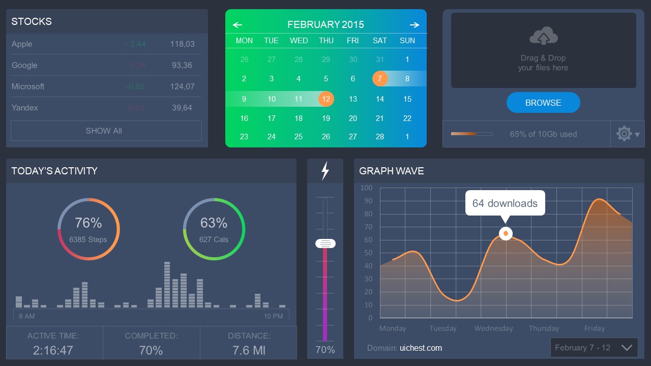
A data dashboard is a visual tool for analyzing information. Different graphs, charts, and tables are consolidated in a layout to showcase the information required to achieve one or more objectives. Dashboards help quickly see Key Performance Indicators (KPIs). You don’t make new visuals in the dashboard; instead, you use it to display visuals you’ve already made in worksheets [3] .
Keeping the number of visuals on a dashboard to three or four is recommended. Adding too many can make it hard to see the main points [4]. Dashboards can be used for business analytics to analyze sales, revenue, and marketing metrics at a time. They are also used in the manufacturing industry, as they allow users to grasp the entire production scenario at the moment while tracking the core KPIs for each line.
Real-Life Application of a Dashboard
Consider a project manager presenting a software development project’s progress to a tech company’s leadership team. He follows the following steps.
Step 1: Defining Key Metrics
To effectively communicate the project’s status, identify key metrics such as completion status, budget, and bug resolution rates. Then, choose measurable metrics aligned with project objectives.
Step 2: Choosing Visualization Widgets
After finalizing the data, presentation aids that align with each metric are selected. For this project, the project manager chooses a progress bar for the completion status and uses bar charts for budget allocation. Likewise, he implements line charts for bug resolution rates.

Step 3: Dashboard Layout
Key metrics are prominently placed in the dashboard for easy visibility, and the manager ensures that it appears clean and organized.
Dashboards provide a comprehensive view of key project metrics. Users can interact with data, customize views, and drill down for detailed analysis. However, creating an effective dashboard requires careful planning to avoid clutter. Besides, dashboards rely on the availability and accuracy of underlying data sources.
For more information, check our article on how to design a dashboard presentation , and discover our collection of dashboard PowerPoint templates .
Treemap charts represent hierarchical data structured in a series of nested rectangles [6] . As each branch of the ‘tree’ is given a rectangle, smaller tiles can be seen representing sub-branches, meaning elements on a lower hierarchical level than the parent rectangle. Each one of those rectangular nodes is built by representing an area proportional to the specified data dimension.
Treemaps are useful for visualizing large datasets in compact space. It is easy to identify patterns, such as which categories are dominant. Common applications of the treemap chart are seen in the IT industry, such as resource allocation, disk space management, website analytics, etc. Also, they can be used in multiple industries like healthcare data analysis, market share across different product categories, or even in finance to visualize portfolios.
Real-Life Application of a Treemap Chart
Let’s consider a financial scenario where a financial team wants to represent the budget allocation of a company. There is a hierarchy in the process, so it is helpful to use a treemap chart. In the chart, the top-level rectangle could represent the total budget, and it would be subdivided into smaller rectangles, each denoting a specific department. Further subdivisions within these smaller rectangles might represent individual projects or cost categories.
Step 1: Define Your Data Hierarchy
While presenting data on the budget allocation, start by outlining the hierarchical structure. The sequence will be like the overall budget at the top, followed by departments, projects within each department, and finally, individual cost categories for each project.
- Top-level rectangle: Total Budget
- Second-level rectangles: Departments (Engineering, Marketing, Sales)
- Third-level rectangles: Projects within each department
- Fourth-level rectangles: Cost categories for each project (Personnel, Marketing Expenses, Equipment)
Step 2: Choose a Suitable Tool
It’s time to select a data visualization tool supporting Treemaps. Popular choices include Tableau, Microsoft Power BI, PowerPoint, or even coding with libraries like D3.js. It is vital to ensure that the chosen tool provides customization options for colors, labels, and hierarchical structures.
Here, the team uses PowerPoint for this guide because of its user-friendly interface and robust Treemap capabilities.
Step 3: Make a Treemap Chart with PowerPoint
After opening the PowerPoint presentation, they chose “SmartArt” to form the chart. The SmartArt Graphic window has a “Hierarchy” category on the left. Here, you will see multiple options. You can choose any layout that resembles a Treemap. The “Table Hierarchy” or “Organization Chart” options can be adapted. The team selects the Table Hierarchy as it looks close to a Treemap.
Step 5: Input Your Data
After that, a new window will open with a basic structure. They add the data one by one by clicking on the text boxes. They start with the top-level rectangle, representing the total budget.

Step 6: Customize the Treemap
By clicking on each shape, they customize its color, size, and label. At the same time, they can adjust the font size, style, and color of labels by using the options in the “Format” tab in PowerPoint. Using different colors for each level enhances the visual difference.
Treemaps excel at illustrating hierarchical structures. These charts make it easy to understand relationships and dependencies. They efficiently use space, compactly displaying a large amount of data, reducing the need for excessive scrolling or navigation. Additionally, using colors enhances the understanding of data by representing different variables or categories.
In some cases, treemaps might become complex, especially with deep hierarchies. It becomes challenging for some users to interpret the chart. At the same time, displaying detailed information within each rectangle might be constrained by space. It potentially limits the amount of data that can be shown clearly. Without proper labeling and color coding, there’s a risk of misinterpretation.
A heatmap is a data visualization tool that uses color coding to represent values across a two-dimensional surface. In these, colors replace numbers to indicate the magnitude of each cell. This color-shaded matrix display is valuable for summarizing and understanding data sets with a glance [7] . The intensity of the color corresponds to the value it represents, making it easy to identify patterns, trends, and variations in the data.
As a tool, heatmaps help businesses analyze website interactions, revealing user behavior patterns and preferences to enhance overall user experience. In addition, companies use heatmaps to assess content engagement, identifying popular sections and areas of improvement for more effective communication. They excel at highlighting patterns and trends in large datasets, making it easy to identify areas of interest.
We can implement heatmaps to express multiple data types, such as numerical values, percentages, or even categorical data. Heatmaps help us easily spot areas with lots of activity, making them helpful in figuring out clusters [8] . When making these maps, it is important to pick colors carefully. The colors need to show the differences between groups or levels of something. And it is good to use colors that people with colorblindness can easily see.
Check our detailed guide on how to create a heatmap here. Also discover our collection of heatmap PowerPoint templates .
Pie charts are circular statistical graphics divided into slices to illustrate numerical proportions. Each slice represents a proportionate part of the whole, making it easy to visualize the contribution of each component to the total.
The size of the pie charts is influenced by the value of data points within each pie. The total of all data points in a pie determines its size. The pie with the highest data points appears as the largest, whereas the others are proportionally smaller. However, you can present all pies of the same size if proportional representation is not required [9] . Sometimes, pie charts are difficult to read, or additional information is required. A variation of this tool can be used instead, known as the donut chart , which has the same structure but a blank center, creating a ring shape. Presenters can add extra information, and the ring shape helps to declutter the graph.
Pie charts are used in business to show percentage distribution, compare relative sizes of categories, or present straightforward data sets where visualizing ratios is essential.
Real-Life Application of Pie Charts
Consider a scenario where you want to represent the distribution of the data. Each slice of the pie chart would represent a different category, and the size of each slice would indicate the percentage of the total portion allocated to that category.
Step 1: Define Your Data Structure
Imagine you are presenting the distribution of a project budget among different expense categories.
- Column A: Expense Categories (Personnel, Equipment, Marketing, Miscellaneous)
- Column B: Budget Amounts ($40,000, $30,000, $20,000, $10,000) Column B represents the values of your categories in Column A.
Step 2: Insert a Pie Chart
Using any of the accessible tools, you can create a pie chart. The most convenient tools for forming a pie chart in a presentation are presentation tools such as PowerPoint or Google Slides. You will notice that the pie chart assigns each expense category a percentage of the total budget by dividing it by the total budget.
For instance:
- Personnel: $40,000 / ($40,000 + $30,000 + $20,000 + $10,000) = 40%
- Equipment: $30,000 / ($40,000 + $30,000 + $20,000 + $10,000) = 30%
- Marketing: $20,000 / ($40,000 + $30,000 + $20,000 + $10,000) = 20%
- Miscellaneous: $10,000 / ($40,000 + $30,000 + $20,000 + $10,000) = 10%
You can make a chart out of this or just pull out the pie chart from the data.

3D pie charts and 3D donut charts are quite popular among the audience. They stand out as visual elements in any presentation slide, so let’s take a look at how our pie chart example would look in 3D pie chart format.

Step 03: Results Interpretation
The pie chart visually illustrates the distribution of the project budget among different expense categories. Personnel constitutes the largest portion at 40%, followed by equipment at 30%, marketing at 20%, and miscellaneous at 10%. This breakdown provides a clear overview of where the project funds are allocated, which helps in informed decision-making and resource management. It is evident that personnel are a significant investment, emphasizing their importance in the overall project budget.
Pie charts provide a straightforward way to represent proportions and percentages. They are easy to understand, even for individuals with limited data analysis experience. These charts work well for small datasets with a limited number of categories.
However, a pie chart can become cluttered and less effective in situations with many categories. Accurate interpretation may be challenging, especially when dealing with slight differences in slice sizes. In addition, these charts are static and do not effectively convey trends over time.
For more information, check our collection of pie chart templates for PowerPoint .
Histograms present the distribution of numerical variables. Unlike a bar chart that records each unique response separately, histograms organize numeric responses into bins and show the frequency of reactions within each bin [10] . The x-axis of a histogram shows the range of values for a numeric variable. At the same time, the y-axis indicates the relative frequencies (percentage of the total counts) for that range of values.
Whenever you want to understand the distribution of your data, check which values are more common, or identify outliers, histograms are your go-to. Think of them as a spotlight on the story your data is telling. A histogram can provide a quick and insightful overview if you’re curious about exam scores, sales figures, or any numerical data distribution.
Real-Life Application of a Histogram
In the histogram data analysis presentation example, imagine an instructor analyzing a class’s grades to identify the most common score range. A histogram could effectively display the distribution. It will show whether most students scored in the average range or if there are significant outliers.
Step 1: Gather Data
He begins by gathering the data. The scores of each student in class are gathered to analyze exam scores.
| Names | Score |
|---|---|
| Alice | 78 |
| Bob | 85 |
| Clara | 92 |
| David | 65 |
| Emma | 72 |
| Frank | 88 |
| Grace | 76 |
| Henry | 95 |
| Isabel | 81 |
| Jack | 70 |
| Kate | 60 |
| Liam | 89 |
| Mia | 75 |
| Noah | 84 |
| Olivia | 92 |
After arranging the scores in ascending order, bin ranges are set.
Step 2: Define Bins
Bins are like categories that group similar values. Think of them as buckets that organize your data. The presenter decides how wide each bin should be based on the range of the values. For instance, the instructor sets the bin ranges based on score intervals: 60-69, 70-79, 80-89, and 90-100.
Step 3: Count Frequency
Now, he counts how many data points fall into each bin. This step is crucial because it tells you how often specific ranges of values occur. The result is the frequency distribution, showing the occurrences of each group.
Here, the instructor counts the number of students in each category.
- 60-69: 1 student (Kate)
- 70-79: 4 students (David, Emma, Grace, Jack)
- 80-89: 7 students (Alice, Bob, Frank, Isabel, Liam, Mia, Noah)
- 90-100: 3 students (Clara, Henry, Olivia)
Step 4: Create the Histogram
It’s time to turn the data into a visual representation. Draw a bar for each bin on a graph. The width of the bar should correspond to the range of the bin, and the height should correspond to the frequency. To make your histogram understandable, label the X and Y axes.
In this case, the X-axis should represent the bins (e.g., test score ranges), and the Y-axis represents the frequency.

The histogram of the class grades reveals insightful patterns in the distribution. Most students, with seven students, fall within the 80-89 score range. The histogram provides a clear visualization of the class’s performance. It showcases a concentration of grades in the upper-middle range with few outliers at both ends. This analysis helps in understanding the overall academic standing of the class. It also identifies the areas for potential improvement or recognition.
Thus, histograms provide a clear visual representation of data distribution. They are easy to interpret, even for those without a statistical background. They apply to various types of data, including continuous and discrete variables. One weak point is that histograms do not capture detailed patterns in students’ data, with seven compared to other visualization methods.
A scatter plot is a graphical representation of the relationship between two variables. It consists of individual data points on a two-dimensional plane. This plane plots one variable on the x-axis and the other on the y-axis. Each point represents a unique observation. It visualizes patterns, trends, or correlations between the two variables.
Scatter plots are also effective in revealing the strength and direction of relationships. They identify outliers and assess the overall distribution of data points. The points’ dispersion and clustering reflect the relationship’s nature, whether it is positive, negative, or lacks a discernible pattern. In business, scatter plots assess relationships between variables such as marketing cost and sales revenue. They help present data correlations and decision-making.
Real-Life Application of Scatter Plot
A group of scientists is conducting a study on the relationship between daily hours of screen time and sleep quality. After reviewing the data, they managed to create this table to help them build a scatter plot graph:
| Participant ID | Daily Hours of Screen Time | Sleep Quality Rating |
|---|---|---|
| 1 | 9 | 3 |
| 2 | 2 | 8 |
| 3 | 1 | 9 |
| 4 | 0 | 10 |
| 5 | 1 | 9 |
| 6 | 3 | 7 |
| 7 | 4 | 7 |
| 8 | 5 | 6 |
| 9 | 5 | 6 |
| 10 | 7 | 3 |
| 11 | 10 | 1 |
| 12 | 6 | 5 |
| 13 | 7 | 3 |
| 14 | 8 | 2 |
| 15 | 9 | 2 |
| 16 | 4 | 7 |
| 17 | 5 | 6 |
| 18 | 4 | 7 |
| 19 | 9 | 2 |
| 20 | 6 | 4 |
| 21 | 3 | 7 |
| 22 | 10 | 1 |
| 23 | 2 | 8 |
| 24 | 5 | 6 |
| 25 | 3 | 7 |
| 26 | 1 | 9 |
| 27 | 8 | 2 |
| 28 | 4 | 6 |
| 29 | 7 | 3 |
| 30 | 2 | 8 |
| 31 | 7 | 4 |
| 32 | 9 | 2 |
| 33 | 10 | 1 |
| 34 | 10 | 1 |
| 35 | 10 | 1 |
In the provided example, the x-axis represents Daily Hours of Screen Time, and the y-axis represents the Sleep Quality Rating.

The scientists observe a negative correlation between the amount of screen time and the quality of sleep. This is consistent with their hypothesis that blue light, especially before bedtime, has a significant impact on sleep quality and metabolic processes.
There are a few things to remember when using a scatter plot. Even when a scatter diagram indicates a relationship, it doesn’t mean one variable affects the other. A third factor can influence both variables. The more the plot resembles a straight line, the stronger the relationship is perceived [11] . If it suggests no ties, the observed pattern might be due to random fluctuations in data. When the scatter diagram depicts no correlation, whether the data might be stratified is worth considering.
Choosing the appropriate data presentation type is crucial when making a presentation . Understanding the nature of your data and the message you intend to convey will guide this selection process. For instance, when showcasing quantitative relationships, scatter plots become instrumental in revealing correlations between variables. If the focus is on emphasizing parts of a whole, pie charts offer a concise display of proportions. Histograms, on the other hand, prove valuable for illustrating distributions and frequency patterns.
Bar charts provide a clear visual comparison of different categories. Likewise, line charts excel in showcasing trends over time, while tables are ideal for detailed data examination. Starting a presentation on data presentation types involves evaluating the specific information you want to communicate and selecting the format that aligns with your message. This ensures clarity and resonance with your audience from the beginning of your presentation.
1. Fact Sheet Dashboard for Data Presentation
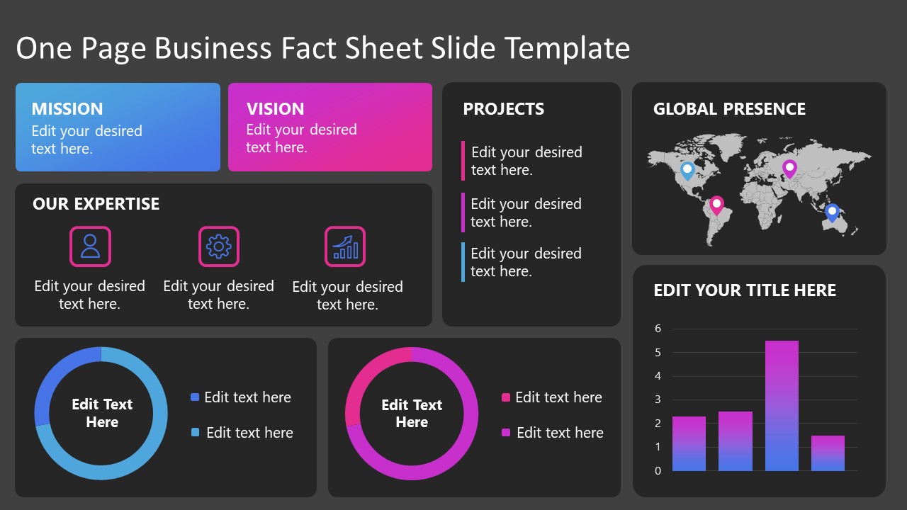
Convey all the data you need to present in this one-pager format, an ideal solution tailored for users looking for presentation aids. Global maps, donut chats, column graphs, and text neatly arranged in a clean layout presented in light and dark themes.
Use This Template
2. 3D Column Chart Infographic PPT Template
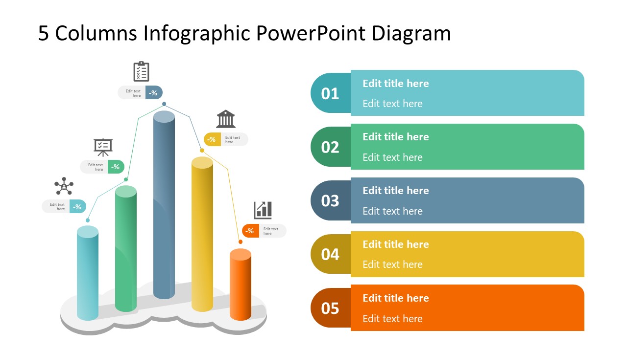
Represent column charts in a highly visual 3D format with this PPT template. A creative way to present data, this template is entirely editable, and we can craft either a one-page infographic or a series of slides explaining what we intend to disclose point by point.
3. Data Circles Infographic PowerPoint Template
An alternative to the pie chart and donut chart diagrams, this template features a series of curved shapes with bubble callouts as ways of presenting data. Expand the information for each arch in the text placeholder areas.
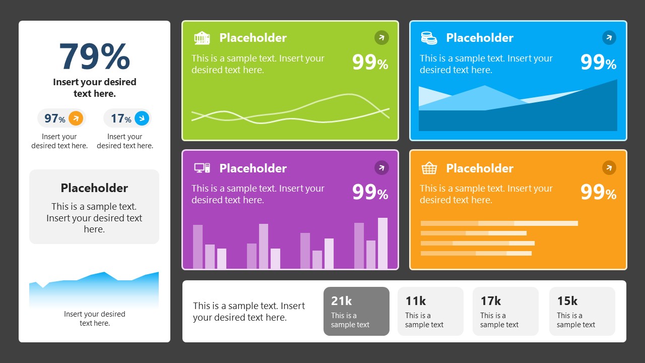
4. Colorful Metrics Dashboard for Data Presentation
This versatile dashboard template helps us in the presentation of the data by offering several graphs and methods to convert numbers into graphics. Implement it for e-commerce projects, financial projections, project development, and more.
5. Animated Data Presentation Tools for PowerPoint & Google Slides

A slide deck filled with most of the tools mentioned in this article, from bar charts, column charts, treemap graphs, pie charts, histogram, etc. Animated effects make each slide look dynamic when sharing data with stakeholders.
6. Statistics Waffle Charts PPT Template for Data Presentations
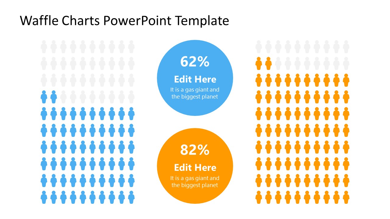
This PPT template helps us how to present data beyond the typical pie chart representation. It is widely used for demographics, so it’s a great fit for marketing teams, data science professionals, HR personnel, and more.
7. Data Presentation Dashboard Template for Google Slides
A compendium of tools in dashboard format featuring line graphs, bar charts, column charts, and neatly arranged placeholder text areas.
8. Weather Dashboard for Data Presentation
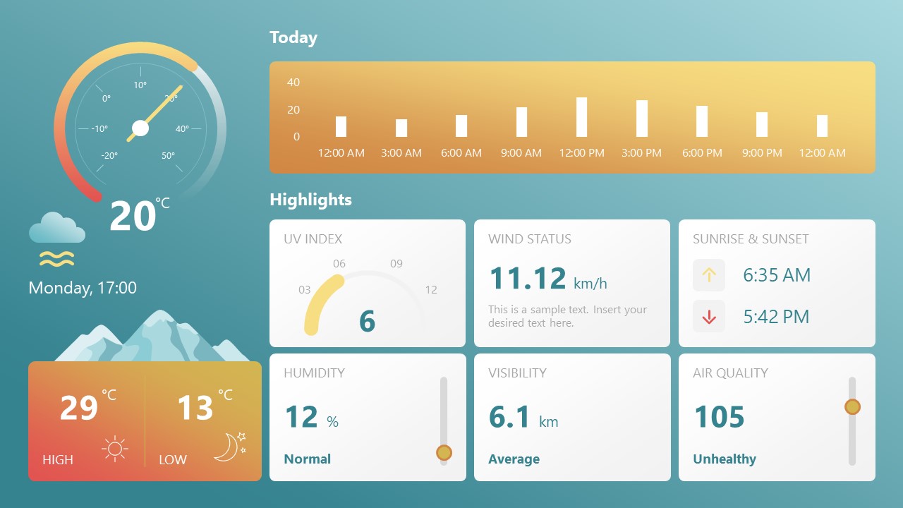
Share weather data for agricultural presentation topics, environmental studies, or any kind of presentation that requires a highly visual layout for weather forecasting on a single day. Two color themes are available.
9. Social Media Marketing Dashboard Data Presentation Template
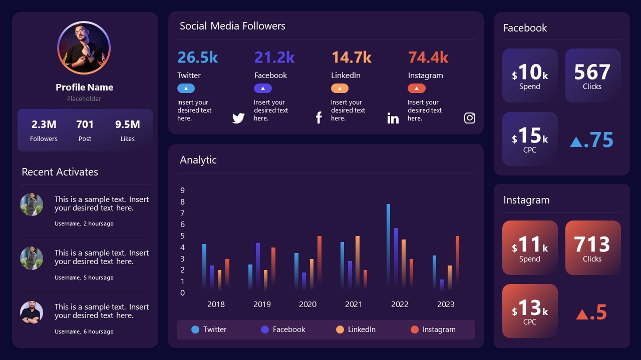
Intended for marketing professionals, this dashboard template for data presentation is a tool for presenting data analytics from social media channels. Two slide layouts featuring line graphs and column charts.
10. Project Management Summary Dashboard Template
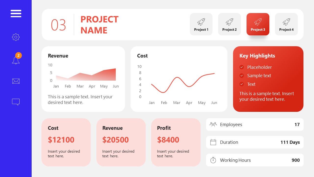
A tool crafted for project managers to deliver highly visual reports on a project’s completion, the profits it delivered for the company, and expenses/time required to execute it. 4 different color layouts are available.
11. Profit & Loss Dashboard for PowerPoint and Google Slides
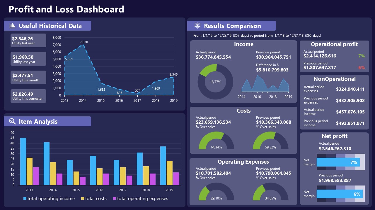
A must-have for finance professionals. This typical profit & loss dashboard includes progress bars, donut charts, column charts, line graphs, and everything that’s required to deliver a comprehensive report about a company’s financial situation.
Overwhelming visuals
One of the mistakes related to using data-presenting methods is including too much data or using overly complex visualizations. They can confuse the audience and dilute the key message.
Inappropriate chart types
Choosing the wrong type of chart for the data at hand can lead to misinterpretation. For example, using a pie chart for data that doesn’t represent parts of a whole is not right.
Lack of context
Failing to provide context or sufficient labeling can make it challenging for the audience to understand the significance of the presented data.
Inconsistency in design
Using inconsistent design elements and color schemes across different visualizations can create confusion and visual disarray.
Failure to provide details
Simply presenting raw data without offering clear insights or takeaways can leave the audience without a meaningful conclusion.
Lack of focus
Not having a clear focus on the key message or main takeaway can result in a presentation that lacks a central theme.
Visual accessibility issues
Overlooking the visual accessibility of charts and graphs can exclude certain audience members who may have difficulty interpreting visual information.
In order to avoid these mistakes in data presentation, presenters can benefit from using presentation templates . These templates provide a structured framework. They ensure consistency, clarity, and an aesthetically pleasing design, enhancing data communication’s overall impact.
Understanding and choosing data presentation types are pivotal in effective communication. Each method serves a unique purpose, so selecting the appropriate one depends on the nature of the data and the message to be conveyed. The diverse array of presentation types offers versatility in visually representing information, from bar charts showing values to pie charts illustrating proportions.
Using the proper method enhances clarity, engages the audience, and ensures that data sets are not just presented but comprehensively understood. By appreciating the strengths and limitations of different presentation types, communicators can tailor their approach to convey information accurately, developing a deeper connection between data and audience understanding.
[1] Government of Canada, S.C. (2021) 5 Data Visualization 5.2 Bar Chart , 5.2 Bar chart . https://www150.statcan.gc.ca/n1/edu/power-pouvoir/ch9/bargraph-diagrammeabarres/5214818-eng.htm
[2] Kosslyn, S.M., 1989. Understanding charts and graphs. Applied cognitive psychology, 3(3), pp.185-225. https://apps.dtic.mil/sti/pdfs/ADA183409.pdf
[3] Creating a Dashboard . https://it.tufts.edu/book/export/html/1870
[4] https://www.goldenwestcollege.edu/research/data-and-more/data-dashboards/index.html
[5] https://www.mit.edu/course/21/21.guide/grf-line.htm
[6] Jadeja, M. and Shah, K., 2015, January. Tree-Map: A Visualization Tool for Large Data. In GSB@ SIGIR (pp. 9-13). https://ceur-ws.org/Vol-1393/gsb15proceedings.pdf#page=15
[7] Heat Maps and Quilt Plots. https://www.publichealth.columbia.edu/research/population-health-methods/heat-maps-and-quilt-plots
[8] EIU QGIS WORKSHOP. https://www.eiu.edu/qgisworkshop/heatmaps.php
[9] About Pie Charts. https://www.mit.edu/~mbarker/formula1/f1help/11-ch-c8.htm
[10] Histograms. https://sites.utexas.edu/sos/guided/descriptive/numericaldd/descriptiven2/histogram/ [11] https://asq.org/quality-resources/scatter-diagram
Like this article? Please share
Data Analysis, Data Science, Data Visualization Filed under Design
Related Articles

Filed under Google Slides Tutorials • June 3rd, 2024
How To Make a Graph on Google Slides
Creating quality graphics is an essential aspect of designing data presentations. Learn how to make a graph in Google Slides with this guide.

Filed under Design • March 27th, 2024
How to Make a Presentation Graph
Detailed step-by-step instructions to master the art of how to make a presentation graph in PowerPoint and Google Slides. Check it out!

Filed under Presentation Ideas • February 12th, 2024
Turning Your Data into Eye-opening Stories
What is Data Storytelling is a question that people are constantly asking now. If you seek to understand how to create a data storytelling ppt that will complete the information for your audience, you should read this blog post.
Leave a Reply
Presentation of Data

Statistics deals with the collection, presentation and analysis of the data, as well as drawing meaningful conclusions from the given data. Generally, the data can be classified into two different types, namely primary data and secondary data. If the information is collected by the investigator with a definite objective in their mind, then the data obtained is called the primary data. If the information is gathered from a source, which already had the information stored, then the data obtained is called secondary data. Once the data is collected, the presentation of data plays a major role in concluding the result. Here, we will discuss how to present the data with many solved examples.
What is Meant by Presentation of Data?
As soon as the data collection is over, the investigator needs to find a way of presenting the data in a meaningful, efficient and easily understood way to identify the main features of the data at a glance using a suitable presentation method. Generally, the data in the statistics can be presented in three different forms, such as textual method, tabular method and graphical method.
Presentation of Data Examples
Now, let us discuss how to present the data in a meaningful way with the help of examples.
Consider the marks given below, which are obtained by 10 students in Mathematics:
36, 55, 73, 95, 42, 60, 78, 25, 62, 75.
Find the range for the given data.
Given Data: 36, 55, 73, 95, 42, 60, 78, 25, 62, 75.
The data given is called the raw data.
First, arrange the data in the ascending order : 25, 36, 42, 55, 60, 62, 73, 75, 78, 95.
Therefore, the lowest mark is 25 and the highest mark is 95.
We know that the range of the data is the difference between the highest and the lowest value in the dataset.
Therefore, Range = 95-25 = 70.
Note: Presentation of data in ascending or descending order can be time-consuming if we have a larger number of observations in an experiment.
Now, let us discuss how to present the data if we have a comparatively more number of observations in an experiment.
Consider the marks obtained by 30 students in Mathematics subject (out of 100 marks)
10, 20, 36, 92, 95, 40, 50, 56, 60, 70, 92, 88, 80, 70, 72, 70, 36, 40, 36, 40, 92, 40, 50, 50, 56, 60, 70, 60, 60, 88.
In this example, the number of observations is larger compared to example 1. So, the presentation of data in ascending or descending order is a bit time-consuming. Hence, we can go for the method called ungrouped frequency distribution table or simply frequency distribution table . In this method, we can arrange the data in tabular form in terms of frequency.
For example, 3 students scored 50 marks. Hence, the frequency of 50 marks is 3. Now, let us construct the frequency distribution table for the given data.
Therefore, the presentation of data is given as below:
|
| |
|---|---|
| 10 | 1 |
| 20 | 1 |
| 36 | 3 |
| 40 | 4 |
| 50 | 3 |
| 56 | 2 |
| 60 | 4 |
| 70 | 4 |
| 72 | 1 |
| 80 | 1 |
| 88 | 2 |
| 92 | 3 |
| 95 | 1 |
|
|
|
The following example shows the presentation of data for the larger number of observations in an experiment.
Consider the marks obtained by 100 students in a Mathematics subject (out of 100 marks)
95, 67, 28, 32, 65, 65, 69, 33, 98, 96,76, 42, 32, 38, 42, 40, 40, 69, 95, 92, 75, 83, 76, 83, 85, 62, 37, 65, 63, 42, 89, 65, 73, 81, 49, 52, 64, 76, 83, 92, 93, 68, 52, 79, 81, 83, 59, 82, 75, 82, 86, 90, 44, 62, 31, 36, 38, 42, 39, 83, 87, 56, 58, 23, 35, 76, 83, 85, 30, 68, 69, 83, 86, 43, 45, 39, 83, 75, 66, 83, 92, 75, 89, 66, 91, 27, 88, 89, 93, 42, 53, 69, 90, 55, 66, 49, 52, 83, 34, 36.
Now, we have 100 observations to present the data. In this case, we have more data when compared to example 1 and example 2. So, these data can be arranged in the tabular form called the grouped frequency table. Hence, we group the given data like 20-29, 30-39, 40-49, ….,90-99 (As our data is from 23 to 98). The grouping of data is called the “class interval” or “classes”, and the size of the class is called “class-size” or “class-width”.
In this case, the class size is 10. In each class, we have a lower-class limit and an upper-class limit. For example, if the class interval is 30-39, the lower-class limit is 30, and the upper-class limit is 39. Therefore, the least number in the class interval is called the lower-class limit and the greatest limit in the class interval is called upper-class limit.
Hence, the presentation of data in the grouped frequency table is given below:
|
| |
|---|---|
| 20 – 29 | 3 |
| 30 – 39 | 14 |
| 40 – 49 | 12 |
| 50 – 59 | 8 |
| 60 – 69 | 18 |
| 70 – 79 | 10 |
| 80 – 89 | 23 |
| 90 – 99 | 12 |
|
|
|
Hence, the presentation of data in this form simplifies the data and it helps to enable the observer to understand the main feature of data at a glance.
Practice Problems
- The heights of 50 students (in cms) are given below. Present the data using the grouped frequency table by taking the class intervals as 160 -165, 165 -170, and so on. Data: 161, 150, 154, 165, 168, 161, 154, 162, 150, 151, 162, 164, 171, 165, 158, 154, 156, 172, 160, 170, 153, 159, 161, 170, 162, 165, 166, 168, 165, 164, 154, 152, 153, 156, 158, 162, 160, 161, 173, 166, 161, 159, 162, 167, 168, 159, 158, 153, 154, 159.
- Three coins are tossed simultaneously and each time the number of heads occurring is noted and it is given below. Present the data using the frequency distribution table. Data: 0, 1, 2, 2, 1, 2, 3, 1, 3, 0, 1, 3, 1, 1, 2, 2, 0, 1, 2, 1, 3, 0, 0, 1, 1, 2, 3, 2, 2, 0.
To learn more Maths-related concepts, stay tuned with BYJU’S – The Learning App and download the app today!
| MATHS Related Links | |
Leave a Comment Cancel reply
Your Mobile number and Email id will not be published. Required fields are marked *
Request OTP on Voice Call
Post My Comment
Register with BYJU'S & Download Free PDFs
Register with byju's & watch live videos.
- SUGGESTED TOPICS
- The Magazine
- Newsletters
- Managing Yourself
- Managing Teams
- Work-life Balance
- The Big Idea
- Data & Visuals
- Reading Lists
- Case Selections
- HBR Learning
- Topic Feeds
- Account Settings
- Email Preferences
Present Your Data Like a Pro
- Joel Schwartzberg

Demystify the numbers. Your audience will thank you.
While a good presentation has data, data alone doesn’t guarantee a good presentation. It’s all about how that data is presented. The quickest way to confuse your audience is by sharing too many details at once. The only data points you should share are those that significantly support your point — and ideally, one point per chart. To avoid the debacle of sheepishly translating hard-to-see numbers and labels, rehearse your presentation with colleagues sitting as far away as the actual audience would. While you’ve been working with the same chart for weeks or months, your audience will be exposed to it for mere seconds. Give them the best chance of comprehending your data by using simple, clear, and complete language to identify X and Y axes, pie pieces, bars, and other diagrammatic elements. Try to avoid abbreviations that aren’t obvious, and don’t assume labeled components on one slide will be remembered on subsequent slides. Every valuable chart or pie graph has an “Aha!” zone — a number or range of data that reveals something crucial to your point. Make sure you visually highlight the “Aha!” zone, reinforcing the moment by explaining it to your audience.
With so many ways to spin and distort information these days, a presentation needs to do more than simply share great ideas — it needs to support those ideas with credible data. That’s true whether you’re an executive pitching new business clients, a vendor selling her services, or a CEO making a case for change.
- JS Joel Schwartzberg oversees executive communications for a major national nonprofit, is a professional presentation coach, and is the author of Get to the Point! Sharpen Your Message and Make Your Words Matter and The Language of Leadership: How to Engage and Inspire Your Team . You can find him on LinkedIn and X. TheJoelTruth
Partner Center
We use essential cookies to make Venngage work. By clicking “Accept All Cookies”, you agree to the storing of cookies on your device to enhance site navigation, analyze site usage, and assist in our marketing efforts.
Manage Cookies
Cookies and similar technologies collect certain information about how you’re using our website. Some of them are essential, and without them you wouldn’t be able to use Venngage. But others are optional, and you get to choose whether we use them or not.
Strictly Necessary Cookies
These cookies are always on, as they’re essential for making Venngage work, and making it safe. Without these cookies, services you’ve asked for can’t be provided.
Show cookie providers
- Google Login
Functionality Cookies
These cookies help us provide enhanced functionality and personalisation, and remember your settings. They may be set by us or by third party providers.
Performance Cookies
These cookies help us analyze how many people are using Venngage, where they come from and how they're using it. If you opt out of these cookies, we can’t get feedback to make Venngage better for you and all our users.
- Google Analytics
Targeting Cookies
These cookies are set by our advertising partners to track your activity and show you relevant Venngage ads on other sites as you browse the internet.
- Google Tag Manager
- Infographics
- Daily Infographics
- Popular Templates
- Accessibility
- Graphic Design
- Graphs and Charts
- Data Visualization
- Human Resources
- Beginner Guides
Blog Data Visualization 10 Data Presentation Examples For Strategic Communication
10 Data Presentation Examples For Strategic Communication
Written by: Krystle Wong Sep 28, 2023

Knowing how to present data is like having a superpower.
Data presentation today is no longer just about numbers on a screen; it’s storytelling with a purpose. It’s about captivating your audience, making complex stuff look simple and inspiring action.
To help turn your data into stories that stick, influence decisions and make an impact, check out Venngage’s free chart maker or follow me on a tour into the world of data storytelling along with data presentation templates that work across different fields, from business boardrooms to the classroom and beyond. Keep scrolling to learn more!
Click to jump ahead:
10 Essential data presentation examples + methods you should know
What should be included in a data presentation, what are some common mistakes to avoid when presenting data, faqs on data presentation examples, transform your message with impactful data storytelling.
Data presentation is a vital skill in today’s information-driven world. Whether you’re in business, academia, or simply want to convey information effectively, knowing the different ways of presenting data is crucial. For impactful data storytelling, consider these essential data presentation methods:
1. Bar graph
Ideal for comparing data across categories or showing trends over time.
Bar graphs, also known as bar charts are workhorses of data presentation. They’re like the Swiss Army knives of visualization methods because they can be used to compare data in different categories or display data changes over time.
In a bar chart, categories are displayed on the x-axis and the corresponding values are represented by the height of the bars on the y-axis.

It’s a straightforward and effective way to showcase raw data, making it a staple in business reports, academic presentations and beyond.
Make sure your bar charts are concise with easy-to-read labels. Whether your bars go up or sideways, keep it simple by not overloading with too many categories.

2. Line graph
Great for displaying trends and variations in data points over time or continuous variables.
Line charts or line graphs are your go-to when you want to visualize trends and variations in data sets over time.
One of the best quantitative data presentation examples, they work exceptionally well for showing continuous data, such as sales projections over the last couple of years or supply and demand fluctuations.

The x-axis represents time or a continuous variable and the y-axis represents the data values. By connecting the data points with lines, you can easily spot trends and fluctuations.
A tip when presenting data with line charts is to minimize the lines and not make it too crowded. Highlight the big changes, put on some labels and give it a catchy title.

3. Pie chart
Useful for illustrating parts of a whole, such as percentages or proportions.
Pie charts are perfect for showing how a whole is divided into parts. They’re commonly used to represent percentages or proportions and are great for presenting survey results that involve demographic data.
Each “slice” of the pie represents a portion of the whole and the size of each slice corresponds to its share of the total.

While pie charts are handy for illustrating simple distributions, they can become confusing when dealing with too many categories or when the differences in proportions are subtle.
Don’t get too carried away with slices — label those slices with percentages or values so people know what’s what and consider using a legend for more categories.

4. Scatter plot
Effective for showing the relationship between two variables and identifying correlations.
Scatter plots are all about exploring relationships between two variables. They’re great for uncovering correlations, trends or patterns in data.
In a scatter plot, every data point appears as a dot on the chart, with one variable marked on the horizontal x-axis and the other on the vertical y-axis.

By examining the scatter of points, you can discern the nature of the relationship between the variables, whether it’s positive, negative or no correlation at all.
If you’re using scatter plots to reveal relationships between two variables, be sure to add trendlines or regression analysis when appropriate to clarify patterns. Label data points selectively or provide tooltips for detailed information.

5. Histogram
Best for visualizing the distribution and frequency of a single variable.
Histograms are your choice when you want to understand the distribution and frequency of a single variable.
They divide the data into “bins” or intervals and the height of each bar represents the frequency or count of data points falling into that interval.

Histograms are excellent for helping to identify trends in data distributions, such as peaks, gaps or skewness.
Here’s something to take note of — ensure that your histogram bins are appropriately sized to capture meaningful data patterns. Using clear axis labels and titles can also help explain the distribution of the data effectively.

6. Stacked bar chart
Useful for showing how different components contribute to a whole over multiple categories.
Stacked bar charts are a handy choice when you want to illustrate how different components contribute to a whole across multiple categories.
Each bar represents a category and the bars are divided into segments to show the contribution of various components within each category.

This method is ideal for highlighting both the individual and collective significance of each component, making it a valuable tool for comparative analysis.
Stacked bar charts are like data sandwiches—label each layer so people know what’s what. Keep the order logical and don’t forget the paintbrush for snazzy colors. Here’s a data analysis presentation example on writers’ productivity using stacked bar charts:

7. Area chart
Similar to line charts but with the area below the lines filled, making them suitable for showing cumulative data.
Area charts are close cousins of line charts but come with a twist.
Imagine plotting the sales of a product over several months. In an area chart, the space between the line and the x-axis is filled, providing a visual representation of the cumulative total.

This makes it easy to see how values stack up over time, making area charts a valuable tool for tracking trends in data.
For area charts, use them to visualize cumulative data and trends, but avoid overcrowding the chart. Add labels, especially at significant points and make sure the area under the lines is filled with a visually appealing color gradient.

8. Tabular presentation
Presenting data in rows and columns, often used for precise data values and comparisons.
Tabular data presentation is all about clarity and precision. Think of it as presenting numerical data in a structured grid, with rows and columns clearly displaying individual data points.
A table is invaluable for showcasing detailed data, facilitating comparisons and presenting numerical information that needs to be exact. They’re commonly used in reports, spreadsheets and academic papers.

When presenting tabular data, organize it neatly with clear headers and appropriate column widths. Highlight important data points or patterns using shading or font formatting for better readability.
9. Textual data
Utilizing written or descriptive content to explain or complement data, such as annotations or explanatory text.
Textual data presentation may not involve charts or graphs, but it’s one of the most used qualitative data presentation examples.
It involves using written content to provide context, explanations or annotations alongside data visuals. Think of it as the narrative that guides your audience through the data.
Well-crafted textual data can make complex information more accessible and help your audience understand the significance of the numbers and visuals.
Textual data is your chance to tell a story. Break down complex information into bullet points or short paragraphs and use headings to guide the reader’s attention.
10. Pictogram
Using simple icons or images to represent data is especially useful for conveying information in a visually intuitive manner.
Pictograms are all about harnessing the power of images to convey data in an easy-to-understand way.
Instead of using numbers or complex graphs, you use simple icons or images to represent data points.
For instance, you could use a thumbs up emoji to illustrate customer satisfaction levels, where each face represents a different level of satisfaction.

Pictograms are great for conveying data visually, so choose symbols that are easy to interpret and relevant to the data. Use consistent scaling and a legend to explain the symbols’ meanings, ensuring clarity in your presentation.

Looking for more data presentation ideas? Use the Venngage graph maker or browse through our gallery of chart templates to pick a template and get started!
A comprehensive data presentation should include several key elements to effectively convey information and insights to your audience. Here’s a list of what should be included in a data presentation:
1. Title and objective
- Begin with a clear and informative title that sets the context for your presentation.
- State the primary objective or purpose of the presentation to provide a clear focus.

2. Key data points
- Present the most essential data points or findings that align with your objective.
- Use charts, graphical presentations or visuals to illustrate these key points for better comprehension.

3. Context and significance
- Provide a brief overview of the context in which the data was collected and why it’s significant.
- Explain how the data relates to the larger picture or the problem you’re addressing.
4. Key takeaways
- Summarize the main insights or conclusions that can be drawn from the data.
- Highlight the key takeaways that the audience should remember.
5. Visuals and charts
- Use clear and appropriate visual aids to complement the data.
- Ensure that visuals are easy to understand and support your narrative.

6. Implications or actions
- Discuss the practical implications of the data or any recommended actions.
- If applicable, outline next steps or decisions that should be taken based on the data.

7. Q&A and discussion
- Allocate time for questions and open discussion to engage the audience.
- Address queries and provide additional insights or context as needed.
Presenting data is a crucial skill in various professional fields, from business to academia and beyond. To ensure your data presentations hit the mark, here are some common mistakes that you should steer clear of:
Overloading with data
Presenting too much data at once can overwhelm your audience. Focus on the key points and relevant information to keep the presentation concise and focused. Here are some free data visualization tools you can use to convey data in an engaging and impactful way.
Assuming everyone’s on the same page
It’s easy to assume that your audience understands as much about the topic as you do. But this can lead to either dumbing things down too much or diving into a bunch of jargon that leaves folks scratching their heads. Take a beat to figure out where your audience is coming from and tailor your presentation accordingly.
Misleading visuals
Using misleading visuals, such as distorted scales or inappropriate chart types can distort the data’s meaning. Pick the right data infographics and understandable charts to ensure that your visual representations accurately reflect the data.
Not providing context
Data without context is like a puzzle piece with no picture on it. Without proper context, data may be meaningless or misinterpreted. Explain the background, methodology and significance of the data.
Not citing sources properly
Neglecting to cite sources and provide citations for your data can erode its credibility. Always attribute data to its source and utilize reliable sources for your presentation.
Not telling a story
Avoid simply presenting numbers. If your presentation lacks a clear, engaging story that takes your audience on a journey from the beginning (setting the scene) through the middle (data analysis) to the end (the big insights and recommendations), you’re likely to lose their interest.
Infographics are great for storytelling because they mix cool visuals with short and sweet text to explain complicated stuff in a fun and easy way. Create one with Venngage’s free infographic maker to create a memorable story that your audience will remember.
Ignoring data quality
Presenting data without first checking its quality and accuracy can lead to misinformation. Validate and clean your data before presenting it.
Simplify your visuals
Fancy charts might look cool, but if they confuse people, what’s the point? Go for the simplest visual that gets your message across. Having a dilemma between presenting data with infographics v.s data design? This article on the difference between data design and infographics might help you out.
Missing the emotional connection
Data isn’t just about numbers; it’s about people and real-life situations. Don’t forget to sprinkle in some human touch, whether it’s through relatable stories, examples or showing how the data impacts real lives.
Skipping the actionable insights
At the end of the day, your audience wants to know what they should do with all the data. If you don’t wrap up with clear, actionable insights or recommendations, you’re leaving them hanging. Always finish up with practical takeaways and the next steps.
Can you provide some data presentation examples for business reports?
Business reports often benefit from data presentation through bar charts showing sales trends over time, pie charts displaying market share,or tables presenting financial performance metrics like revenue and profit margins.
What are some creative data presentation examples for academic presentations?
Creative data presentation ideas for academic presentations include using statistical infographics to illustrate research findings and statistical data, incorporating storytelling techniques to engage the audience or utilizing heat maps to visualize data patterns.
What are the key considerations when choosing the right data presentation format?
When choosing a chart format , consider factors like data complexity, audience expertise and the message you want to convey. Options include charts (e.g., bar, line, pie), tables, heat maps, data visualization infographics and interactive dashboards.
Knowing the type of data visualization that best serves your data is just half the battle. Here are some best practices for data visualization to make sure that the final output is optimized.
How can I choose the right data presentation method for my data?
To select the right data presentation method, start by defining your presentation’s purpose and audience. Then, match your data type (e.g., quantitative, qualitative) with suitable visualization techniques (e.g., histograms, word clouds) and choose an appropriate presentation format (e.g., slide deck, report, live demo).
For more presentation ideas , check out this guide on how to make a good presentation or use a presentation software to simplify the process.
How can I make my data presentations more engaging and informative?
To enhance data presentations, use compelling narratives, relatable examples and fun data infographics that simplify complex data. Encourage audience interaction, offer actionable insights and incorporate storytelling elements to engage and inform effectively.
The opening of your presentation holds immense power in setting the stage for your audience. To design a presentation and convey your data in an engaging and informative, try out Venngage’s free presentation maker to pick the right presentation design for your audience and topic.
What is the difference between data visualization and data presentation?
Data presentation typically involves conveying data reports and insights to an audience, often using visuals like charts and graphs. Data visualization , on the other hand, focuses on creating those visual representations of data to facilitate understanding and analysis.
Now that you’ve learned a thing or two about how to use these methods of data presentation to tell a compelling data story , it’s time to take these strategies and make them your own.
But here’s the deal: these aren’t just one-size-fits-all solutions. Remember that each example we’ve uncovered here is not a rigid template but a source of inspiration. It’s all about making your audience go, “Wow, I get it now!”
Think of your data presentations as your canvas – it’s where you paint your story, convey meaningful insights and make real change happen.
So, go forth, present your data with confidence and purpose and watch as your strategic influence grows, one compelling presentation at a time.
Discover popular designs

Infographic maker

Brochure maker

White paper online

Newsletter creator

Flyer maker
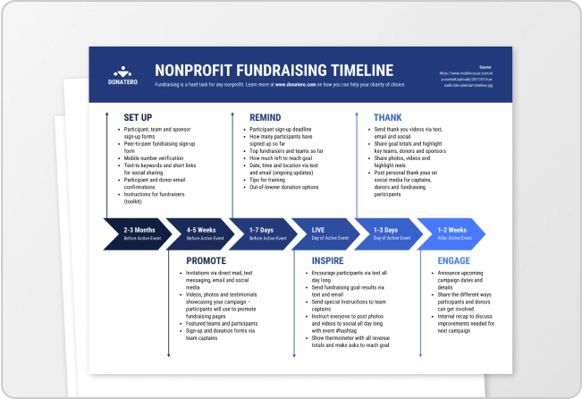
Timeline maker

Letterhead maker
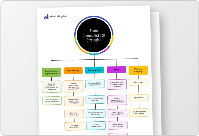
Mind map maker

Ebook maker
Unsupported browser
This site was designed for modern browsers and tested with Internet Explorer version 10 and later.
It may not look or work correctly on your browser.
- Presentations
How to Present Data & Numbers in Presentations (Like a Pro)
Data is more important than ever. But do you know how to present data? Your audience needs information in a way that's easy-to-follow. With charts and graphs, data comes to life.

In this tutorial, you'll learn how to present data. The intuitive presentation of data and information is essential so that your point comes across. With our tips, we'll help you take flat data tables and convert them to useful and explanatory charts.
Why Present Data and Numbers With Charts?
Often, you’ll find yourself presenting data in PowerPoint. It’s a useful tool to illustrate data and bring numbers to life. But if you go about it the wrong way, you’ll distract and confuse your audience. Remember, the goal of sharing data is to deliver insights.
When you think of how to present data, you've got several options. Words alone should be an automatic no-no. Clustering numerical data in text paragraphs will confuse an audience. Similarly, tables don’t go far enough.
Consider the example below. While this approach may work for a simple dataset, it’s hard to capture value insights at a glance. Keep in mind, you want a viewer to quickly grasp the fundamental meaning of the data instantly.

That’s why your best option is to present data and numbers with charts. These are two related ways to present data that take a truly visual approach. Charts and graphs are forms of infographics. An infographic is a visual illustration meant to show ideas. They look great, they're easy to read, and they work.
Recent research vividly shows their effectiveness. Infographics are read at a rate of 30:1 over text articles. Pair this with the fact that visual information represents 90% of what transmits to a reader’s brain . Clearly, these are tools to keep in your wheelhouse.
As you can see below, the table data above transforms from a complex table to a clear and concise visual. It’s the identical range of data! The magic happens in the display of it. Charts are the key to success in the presentation of data and information.

How to Present Data and Numbers in Presentations
We’ve learned that the best way to present data is with charts. Now that you’re armed with this knowledge, you've got many options to choose from.
Premium PowerPoint data presentation templates are your best friend. These take the hard work out of building and sharing data charts. They teach you how to present data in presentations with pre-built options. All you need is your dataset!
For our walkthrough tutorial, we’ll use the Chart Presentation template from Envato Elements. It’s a premium option with 24 custom slide designs inside. Each is easy to customize to meet your data presentation needs.

With the template downloaded and opened in PowerPoint, let’s get to work learning how to present data. Follow the principles below, and you’ll be ready to get started!
1. Assess Your Data
Charts come in all shapes and sizes. There are pie charts, column charts, line charts, and many more. All have many uses, but each is targeted towards different types of data. First, you’ll want to assess the data that you have, and how it would best be presented visually. Let’s work with a sample dataset like the one below.
As you can see, the data has several rows, each representing a different country. Beside these are three columns, each covering sales for a given year. In short, you’re looking at three years of sales forecasts for five countries.

Reading over the data, it’s tough to instantly gain any insights. Sure, if you look long enough, trends start to emerge. But this is a slow, manual process. And imagine if there were fifty countries and twelve years, for example!
Manual analysis would become nearly impossible in a presentation setting. But by using a chart, you can instantly illustrate trends and forecasts. Any viewer – even an untrained eye – can readily see all key points with a moment’s glance.
2. Choose a Visual
Now that you’ve analyzed your data, you can easily see that a chart is essential. But what kind? We briefly mentioned three styles of charts. When you think of how to present data in presentation form, the trick is to choose the style that best fits your data.
For our example, we’re looking at multiple data points for several categories. Here, these data points are three sales values, for five countries each. Keep these ideas for how to present numbers in mind:
- A logical visual would group each country together.
- Then, show each of the three sales figures side by side.
- You could also reverse it – group the years and show sales for all five countries.
In a case like this, a column chart is the ideal choice. These group data just as described.

But when might a different chart type be useful? Imagine if your data included details about Germany’s 2024 sales, for example. Suppose you’re presenting to your marketing team, and they’ve asked how sales of each individual product make up the total. Here, a pie chart would be the perfect option. These show how individual pieces form a whole.
But in this case, we’ve decided on a column chart. Find one in the deck, and let’s insert it. In our template, slide #15 contains a beautiful chart. It’s already built. All you need to do is add your own data.
To do that, click into the chart area, then right-click. From the menu, choose Edit Data. You’ll see an embedded Microsoft Excel spreadsheet launch right inside of PowerPoint. From here, you can simply replace the existing data with the table you already have. As you work, the chart instantly updates itself to match the new data.

In moments, you’ll be presenting data in PowerPoint with this beautiful chart!
3. Style Your Visual
With your chart placed on the slide, you now have an array of design options. Remember, the goal is to make the chart work perfectly for your own data. These options primarily live on the Chart Design menu, which you can find on PowerPoint’s ribbon. With the chart selected, click on Chart Design.
The template has a beautiful color palette, but you can add your own. It helps to choose a color profile with plenty of contrast. This makes your visual even clearer and easier to read.
To add a new palette, click on the Change Colors drop-down menu. You’ll see an array of color swatches display. Click on one, and it'll apply to your chart.

You can add a new background by launching the Chart Styles section in the center of the Chart Design menu. For example, you can choose one with a gray background to make the colors really stand out on the slide.
Also, it’s possible to add more context to the data. The horizontal axis in our example is clear enough, listing countries. But there isn’t any explanation of what the vertical axis represents, or the colorful bars. Follow these steps:
- Open the Add Chart Element dropdown near the upper left of the ribbon.
- Click Axis Titles.
- Choose Primary Vertical.
- You’ll see Axis Title appear on the chart. This is a text box, which you can select and type into.

Finally, back on the Add Chart Element dropdown, choose Legend , and pick a location like Top . Three colorful squares listing the three years shown in the chart will be added to the drawing. These labels aid in the presentation of data and information.
It’s easy to see how to present numbers in chart form, using PowerPoint. Start with a premium template like this, and then customize the chart inside to fit your needs.
4. Add Notes Where Needed
You now know well that charts are the best way to present data. But they don’t have to stand on their own!
Often, it’s useful to add more context. Audiences may understand the data perfectly but have questions. For example: Why are sales for one country climbing, while they are falling in another?
By adding notes where needed, you can add supporting details. It’s best to keep these off of the chart itself. If you clutter up your visual, the value of it diminishes rapidly. Check out an improved example below.

On our slide example, the paragraph section on the left may become a series of quick bullet points. These add supporting details that more fully explain the data shown in the chart.
Again, you may not always need to do this. But never think that a chart must be all-encompassing, explaining every piece of information by itself. The trick is to boost understanding, while remaining clear and concise.
5. Consider an Appendix
You may have extra details that you need to include in your slides.
In our example, imagine that you've got three sales offices in each of the five countries featured. Each of the fifteen makes up a certain percentage of overall sales. This may be key data for your audience, but it would complicate the visual that you just created.
Here, it’s a good idea to add an appendix. An appendix (often at the end of your slide deck) includes more detailed data. You might not review it with a live audience, but they can look at it later in a handout or digital format.
To add an appendix, go to the end of your presentation, and click New Slide on the Home tab. Here, it might be appropriate to share the detailed data in the form of a table. Or, you can add a pie chart, suitable for this style of dataset.

To add a chart from scratch, go to the Insert tab, then choose Chart > Pie. The embedded Excel window will return, and again, you can insert your data.
An appendix may not always be necessary. But you should include one (or more) if you've got meaningful data that you aren’t placing into the main slide deck.
The Best Source for Data Presentation Templates (With Unlimited Downloads)
Envato Elements is the best place to find top data presentation templates . For a low monthly rate, you've got access to unlimited downloads of PPT chart templates. You can try as many as you want, finding those that work best for you.
Explore PowerPoint Chart Templates

And that isn’t all. As an Elements member, you also have unlimited access to stock photos, music, fonts, and more. These are digital assets that pair perfectly with your data presentation.
Elements is an unbeatable offer because of the unlimited flexibility. With premium templates, you gain access to powerful features not found in free designs:
- beautiful data visuals that are pre-built and ready to customize
- stylish, custom fonts to help text stand out
- media placeholders to add supporting images and videos
- fully flexible layouts that adapt to your data and other content
The advantages are many. You save hard work, by leaving the slide design tasks to experts. This gives you the time needed to refine your message. Plus, the finished product will wow any audience, thanks to the expertly-crafted graphics . Truly, Envato Elements is the best value for creatives today.
Need a template, but don't want an unlimited subscription? We've got you covered with templates from GraphicRiver . You'll pay-as-you-go, and these templates give you everything you need. They've got pre-made designs for the best way to present data with less work than ever before.
Now Practice the Best Way to Present Data in Presentations
You just learned new ways to present data. Essentially, you saw how to present data in presentations so that your audience can understand it. Great presenters think of the audience first. They'll thank you for your thoughtful work in how to present numbers and more.
Now, it's your turn! Put these tips on how to present data in presentations to work. Take a flat table in a presentation and convert it with our tips for presenting data in PowerPoint. Just download a template and get started.

9 Data Presentation Tools for Business Success
- By Judhajit Sen
- May 29, 2024
A data presentation is a slide deck that shares quantitative information with an audience using visuals and effective presentation techniques . The goal is to make complex data easily understandable and actionable using data presentation examples like graphs and charts, tables, dashboards, and clear text explanations.
Data presentations help highlight trends, patterns, and insights, allowing the audience to grasp complicated concepts or trends quickly. This makes it easier for them to make informed decisions or conduct deeper analysis.
Data visualization in presentations is used in every field, from academia to business and industry. Raw data is often too complex to understand directly, so data analysis breaks it down into charts and graphs. These tools help turn raw data into useful information.
Once the information is extracted, it’s presented graphically. A good presentation can significantly enhance understanding and response.
Think of data presentation as storytelling in business presentations with charts. A common mistake is assuming the audience understands the data as well as the presenter. Always consider your audience’s knowledge level and what information they need when you present your data.
To present the data effectively:
1. Provide context to help the audience understand the numbers.
2. Compare data groups using visual aids.
3. Step back and view the data from the audience’s perspective.
Data presentations are crucial in nearly every industry, helping professionals share their findings clearly after analyzing data.
Key Takeaways
- Simplifying Complex Data: Data presentations turn complex data into easy-to-understand visuals and narratives, helping audiences quickly grasp trends and insights for informed decision-making.
- Versatile Tools: Various tools like bar charts, dashboards, pie charts, histograms, scatter plots, pictograms, textual presentations, and tables each serve unique purposes, enhancing the clarity and impact of the data.
- Audience Consideration: Tailor your presentation to the audience’s knowledge level, providing context and using simple visuals to make the information accessible and actionable.
- Effective Data Storytelling: Combining clear context, organized visuals, and thoughtful presentation ensures that the data’s story is conveyed effectively, supporting better business decisions and success.
Following are 9 data presentation tools for business success.

Bar charts are a simple yet powerful method of presentation of the data using rectangular bars to show quantities or frequencies. They make it easy to spot patterns or trends at a glance. Bar charts can be vertical (column charts) or horizontal, depending on how you want to display your data.
In a bar graph, categories are displayed on one axis, usually the x-axis for vertical charts and the y-axis for horizontal ones. The bars’ lengths represent the values or frequencies of these categories, with the scale marked on the opposite axis.
These charts are ideal for comparing data across different categories or showing trends over time. Each bar’s height (or length in a horizontal chart) is directly proportional to the value it represents. This visual representation helps illustrate differences or changes in data.
Bar charts are versatile tools in business reports, academic presentations, and more. To make your bar charts effective:
- Ensure they are concise and have easy-to-read labels.
- Avoid clutter by not including too many categories, making the chart hard to read.
- Keep it simple to maintain clarity and impact, whether your bars go up or sideways.
Line Graphs

Line graphs show how data changes over time or with continuous variables. They connect points of data with straight lines, making it easy to see trends and fluctuations. These graphs are handy when comparing multiple datasets over the same timeline.
Using line graphs, you can track things like stock prices, sales projections, or experimental results. The x-axis represents time or another continuous variable, while the y-axis shows the data values. This setup allows you to understand the ups and downs in the data quickly.
To make your graphs effective, keep them simple. Avoid overcrowding with too many lines, highlight significant changes, use labels, and give your graph a clear, catchy title. This will help your audience grasp the information quickly and easily.

A data dashboard is a data analysis presentation example for analyzing information. It combines different graphs, charts, and tables in one layout to show the information needed to meet one or more objectives. Dashboards help quickly see Key Performance Indicators (KPIs) by displaying visuals you’ve already made in worksheets.
It’s best to keep the number of visuals on a dashboard to three or four. Adding too many can make it hard to see the main points. Dashboards are helpful for business analytics, like analyzing sales, revenue, and marketing metrics. In manufacturing, they help users understand the production scenario and track critical KPIs for each production line.
Dashboards represent vital points of data or metrics in an easy-to-understand way. They are often an interactive presentation idea , allowing users to drill down into the data or view different aspects of it.

Pie charts are circular graphs divided into parts to show numerical proportions. Each portion represents a part of the whole, making it easy to see each component’s contribution to the total.
The size of each slice is determined by its value relative to the total. A pie chart with more significant points of data will have larger slices, and the whole chart will be more important. However, you can make all pies the same size if proportional representation isn’t necessary.
Pie charts are helpful in business to show percentage distributions, compare category sizes, or present simple data sets where visualizing ratios is essential. They work best with fewer variables. For more variables, it’s better to use a pie chart calculator that helps to create pie charts easily for various data sets with different color slices.
Each “slice” represents a fraction of the total, and the size of each slice shows its share of the whole. Pie charts are excellent for showing how a whole is divided into parts, such as survey results or demographic data.
While pie charts are great for simple distributions, they can get confusing with too many categories or slight differences in proportions. To keep things clear, label each slice with percentages or values and use a legend if there are many categories. If more detail is needed, consider using a donut chart with a blank center for extra information and a less cluttered look.

A histogram is a graphical presentation of data to help in understanding the distribution of numerical values. Unlike bar charts that show each response separately, histograms group numeric responses into bins and display the frequency of reactions within each bin. The x-axis denotes the range of values, while the y-axis shows the frequency of those values.
Histograms are useful for understanding your data’s distribution, identifying shared values, and spotting outliers. They highlight the story your data tells, whether it’s exam scores, sales figures, or any other numerical data.
Histograms are great for visualizing the distribution and frequency of a single variable. They divide the data into bins, and the height of each bar indicates how many points of data fall into that bin. This makes it easy to see trends like peaks, gaps, or skewness in your data.
To make your histogram effective, choose bin sizes that capture meaningful patterns. Clear axis labels and titles also help in explaining the data distribution.
Scatter Plot

Using individual data points, a scatter plot chart is a presentation of data in visual form to show the relationship between two variables. Each variable is plotted along the x-axis and y-axis, respectively. Each point on the scatter plot represents a single observation.
Scatter plots help visualize patterns, trends, and correlations between the two variables. They can also help identify outliers and understand the overall distribution of data points. The way the points are spread out or clustered together can indicate whether there is a positive, negative, or no clear relationship between the variables.
Scatter plots can be used in practical applications, such as in business, to show how variables like marketing cost and sales revenue are related. They help understand data correlations, which aids in decision-making.
To make scatter plots more effective, consider adding trendlines or regression analysis to highlight patterns. Labeling key data points or tooltips can provide additional information and make the chart easier to interpret.

A pictogram is the simplest form of data presentation and analysis, often used in schools and universities to help students grasp concepts more effectively through pictures.
This type of diagram uses images to represent data. For example, you could draw five books to show the number of books sold in the first week of release, with each image representing 1,000 books. If consumers bought 5,000 books, you would display five book images.
Using simple icons or images makes the information visually intuitive. Instead of relying on numbers or complex graphs, pictograms use straightforward symbols to depict data points. For example, a thumbs-up emoji can illustrate customer satisfaction levels, with each emoji representing a different level of satisfaction.
Pictograms are excellent for visual data presentation. Choose symbols that are easy to interpret and relevant to the data to ensure clarity. Consistent scaling and a legend explaining the symbols’ meanings are essential for an effective presentation.
Textual Presentation

Textual presentation uses words to describe the relationships between pieces of information. This method helps share details that can’t be shown in a graph or table. For example, researchers often present findings in a study textually to provide extra context or explanation. A textual presentation can make the information more transparent.
This type of presentation is common in research and for introducing new ideas. Unlike charts or graphs, it relies solely on paragraphs and words.
Textual presentation also involves using written content, such as annotations or explanatory text, to explain or complement data. While it doesn’t use visual presentation aids like charts, it is a widely used method for presenting qualitative data. Think of it as the narrative that guides your audience through the data.
Adequate textual data may make complex information more accessible. Breaking down complex details into bullet points or short paragraphs helps your audience understand the significance of numbers and visuals. Headings can guide the reader’s attention and tell a coherent story.
Tabular Presentation

Tabular presentation uses tables to share information by organizing data in rows and columns. This method is useful for comparing data and visualizing information. Researchers often use tables to analyze data in various classifications:
Qualitative classification: This includes qualities like nationality, age, social status, appearance, and personality traits, helping to compare sociological and psychological information.
Quantitative classification: This covers items you can count or number.
Spatial classification: This deals with data based on location, such as information about a city, state, or region.
Temporal classification: This involves time-based data measured in seconds, hours, days, or weeks.
Tables simplify data, making it easily consumable, allow for side-by-side comparisons, and save space in your presentation by condensing information.
Using rows and columns, tabular presentation focuses on clarity and precision. It’s about displaying numerical data in a structured grid, clearly showing individual data points. Tables are invaluable for showcasing detailed data, facilitating comparisons, and presenting exact numerical information. They are commonly used in reports, spreadsheets, and academic papers.
Organize tables neatly with clear headers and appropriate column widths to ensure readability. Highlight important data points or patterns using shading or font formatting. Tables are simple and effective, especially when the audience needs to know precise figures.
Elevate Business Decisions with Effective Data Presentations
Data presentations are essential for transforming complex data into understandable and actionable insights. Data presentations simplify the process of interpreting quantitative information by utilizing data presentation examples like charts, graphs, tables, infographics, dashboards, and clear narratives. This method of storytelling with visuals highlights trends, patterns, and insights, enabling audiences to make informed decisions quickly.
In business, data analysis presentations are invaluable. Different types of presentation tools like bar charts help compare categories and track changes over time, while dashboards consolidate various metrics into a comprehensive view. Pie charts and histograms offer clear views of distributions and proportions, aiding in grasping the bigger picture. Scatter plots reveal relationships between variables, and pictograms make data visually intuitive. Textual presentations and tables provide detailed context and precise figures, which are essential for thorough analysis and comparison.
Consider the audience’s knowledge level to tailor the best way to present data in PowerPoint. Clear context, simple visuals, and thoughtful organization ensure the data’s story is easily understood and impactful. Mastering these nine data presentation types can significantly enhance business success by making data-driven decisions more accessible and practical.
Frequently Asked Questions (FAQs)
1. What is a data presentation?
A data presentation is a slide deck that uses visuals and narrative techniques to make complex data easy to understand and actionable. It includes charts, graphs, tables, infographics, dashboards, and clear text explanations.
2. Why are data presentations important in business?
Data presentations are crucial because they help highlight trends, patterns, and insights, making it easier for the audience to understand complicated concepts. This enables better decision-making and deeper analysis.
3. What types of data presentation tools are commonly used?
Common tools include bar charts, line graphs, dashboards, pie charts, histograms, scatter plots, pictograms, textual presentations, and tables. Each tool has a unique way of representing data to aid understanding.
4. How can I ensure my data presentation is effective?
To ensure effectiveness, provide context, compare data sets using visual aids, consider your audience’s knowledge level, and keep visuals simple. Organizing information thoughtfully and avoiding clutter enhances clarity and impact.
Transform Your Data into Compelling Stories with Prezentium
Unlock the full potential of your business data with Prezentium ‘s expert presentation services. Our AI-powered solutions turn complex data into clear, actionable insights, helping you easily make informed decisions.
Prezentium’s Overnight Presentations ensure you wake up to a stunning, ready-to-use presentation in your inbox by 9:30 am PST. Send your requirements by 5:30 pm PST, and let our team combine business acumen, visual design, and data science to craft a presentation that highlights trends and insights seamlessly.
Our Presentation Specialists transform raw ideas and meeting notes into captivating presentations. Whether you need new designs or bespoke templates, our experts bring your vision to life with precision and creativity.
Enhance your team’s skills with Zenith Learning, our interactive workshops that blend structured problem-solving with visual storytelling. Learn to present data effectively and make a lasting impact in your business communications.
Prezentium’s services are designed to help you make the most of your data, from bar charts to dashboards, ensuring your presentations are informative and visually engaging. Let us help you tell your data’s story in a way that resonates. Contact Prezentium today to elevate your business presentations.
Why wait? Avail a complimentary 1-on-1 session with our presentation expert. See how other enterprise leaders are creating impactful presentations with us.
Bad PowerPoint: 6 Poor PowerPoint Slide Practices to Avoid
Greatest sales deck ever: pitch deck tips, 8 tips on how to write a sponsorship proposal template.
A Guide to Effective Data Presentation
Key objectives of data presentation, charts and graphs for great visuals, storytelling with data, visuals, and text, audiences and data presentation, the main idea in data presentation, storyboarding and data presentation, additional resources, data presentation.
Tools for effective data presentation
Financial analysts are required to present their findings in a neat, clear, and straightforward manner. They spend most of their time working with spreadsheets in MS Excel, building financial models , and crunching numbers. These models and calculations can be pretty extensive and complex and may only be understood by the analyst who created them. Effective data presentation skills are critical for being a world-class financial analyst .

It is the analyst’s job to effectively communicate the output to the target audience, such as the management team or a company’s external investors. This requires focusing on the main points, facts, insights, and recommendations that will prompt the necessary action from the audience.
One challenge is making intricate and elaborate work easy to comprehend through great visuals and dashboards. For example, tables, graphs, and charts are tools that an analyst can use to their advantage to give deeper meaning to a company’s financial information. These tools organize relevant numbers that are rather dull and give life and story to them.
Here are some key objectives to think about when presenting financial analysis:
- Visual communication
- Audience and context
- Charts, graphs, and images
- Focus on important points
- Design principles
- Storytelling
- Persuasiveness
For a breakdown of these objectives, check out Excel Dashboards & Data Visualization course to help you become a world-class financial analyst.
Charts and graphs make any financial analysis readable, easy to follow, and provide great data presentation. They are often included in the financial model’s output, which is essential for the key decision-makers in a company.
The decision-makers comprise executives and managers who usually won’t have enough time to synthesize and interpret data on their own to make sound business decisions. Therefore, it is the job of the analyst to enhance the decision-making process and help guide the executives and managers to create value for the company.
When an analyst uses charts, it is necessary to be aware of what good charts and bad charts look like and how to avoid the latter when telling a story with data.
Examples of Good Charts
As for great visuals, you can quickly see what’s going on with the data presentation, saving you time for deciphering their actual meaning. More importantly, great visuals facilitate business decision-making because their goal is to provide persuasive, clear, and unambiguous numeric communication.
For reference, take a look at the example below that shows a dashboard, which includes a gauge chart for growth rates, a bar chart for the number of orders, an area chart for company revenues, and a line chart for EBITDA margins.
To learn the step-by-step process of creating these essential tools in MS Excel, watch our video course titled “ Excel Dashboard & Data Visualization .” Aside from what is given in the example below, our course will also teach how you can use other tables and charts to make your financial analysis stand out professionally.

Learn how to build the graph above in our Dashboards Course !
Example of Poorly Crafted Charts
A bad chart, as seen below, will give the reader a difficult time to find the main takeaway of a report or presentation, because it contains too many colors, labels, and legends, and thus, will often look too busy. It also doesn’t help much if a chart, such as a pie chart, is displayed in 3D, as it skews the size and perceived value of the underlying data. A bad chart will be hard to follow and understand.

Aside from understanding the meaning of the numbers, a financial analyst must learn to combine numbers and language to craft an effective story. Relying only on data for a presentation may leave your audience finding it difficult to read, interpret, and analyze your data. You must do the work for them, and a good story will be easier to follow. It will help you arrive at the main points faster, rather than just solely presenting your report or live presentation with numbers.
The data can be in the form of revenues, expenses, profits, and cash flow. Simply adding notes, comments, and opinions to each line item will add an extra layer of insight, angle, and a new perspective to the report.
Furthermore, by combining data, visuals, and text, your audience will get a clear understanding of the current situation, past events, and possible conclusions and recommendations that can be made for the future.
The simple diagram below shows the different categories of your audience.

This chart is taken from our course on how to present data .
Internal Audience
An internal audience can either be the executives of the company or any employee who works in that company. For executives, the purpose of communicating a data-filled presentation is to give an update about a certain business activity such as a project or an initiative.
Another important purpose is to facilitate decision-making on managing the company’s operations, growing its core business, acquiring new markets and customers, investing in R&D, and other considerations. Knowing the relevant data and information beforehand will guide the decision-makers in making the right choices that will best position the company toward more success.
External Audience
An external audience can either be the company’s existing clients, where there are projects in progress, or new clients that the company wants to build a relationship with and win new business from. The other external audience is the general public, such as the company’s external shareholders and prospective investors of the company.
When it comes to winning new business, the analyst’s presentation will be more promotional and sales-oriented, whereas a project update will contain more specific information for the client, usually with lots of industry jargon.
Audiences for Live and Emailed Presentation
A live presentation contains more visuals and storytelling to connect more with the audience. It must be more precise and should get to the point faster and avoid long-winded speech or text because of limited time.
In contrast, an emailed presentation is expected to be read, so it will include more text. Just like a document or a book, it will include more detailed information, because its context will not be explained with a voice-over as in a live presentation.
When it comes to details, acronyms, and jargon in the presentation, these things depend on whether your audience are experts or not.
Every great presentation requires a clear “main idea”. It is the core purpose of the presentation and should be addressed clearly. Its significance should be highlighted and should cause the targeted audience to take some action on the matter.
An example of a serious and profound idea is given below.

To communicate this big idea, we have to come up with appropriate and effective visual displays to show both the good and bad things surrounding the idea. It should put emphasis and attention on the most important part, which is the critical cash balance and capital investment situation for next year. This is an important component of data presentation.
The storyboarding below is how an analyst would build the presentation based on the big idea. Once the issue or the main idea has been introduced, it will be followed by a demonstration of the positive aspects of the company’s performance, as well as the negative aspects, which are more important and will likely require more attention.
Various ideas will then be suggested to solve the negative issues. However, before choosing the best option, a comparison of the different outcomes of the suggested ideas will be performed. Finally, a recommendation will be made that centers around the optimal choice to address the imminent problem highlighted in the big idea.

This storyboard is taken from our course on how to present data .
To get to the final point (recommendation), a great deal of analysis has been performed, which includes the charts and graphs discussed earlier, to make the whole presentation easy to follow, convincing, and compelling for your audience.
CFI offers the Business Intelligence & Data Analyst (BIDA)® certification program for those looking to take their careers to the next level. To keep learning and developing your knowledge base, please explore the additional relevant resources below:
- Investment Banking Pitch Books
- Excel Dashboards
- Financial Modeling Guide
- Startup Pitch Book
- See all business intelligence resources
- Share this article

Create a free account to unlock this Template
Access and download collection of free Templates to help power your productivity and performance.
Already have an account? Log in
Supercharge your skills with Premium Templates
Take your learning and productivity to the next level with our Premium Templates.
Upgrading to a paid membership gives you access to our extensive collection of plug-and-play Templates designed to power your performance—as well as CFI's full course catalog and accredited Certification Programs.
Already have a Self-Study or Full-Immersion membership? Log in
Access Exclusive Templates
Gain unlimited access to more than 250 productivity Templates, CFI's full course catalog and accredited Certification Programs, hundreds of resources, expert reviews and support, the chance to work with real-world finance and research tools, and more.
Already have a Full-Immersion membership? Log in
- Slidesgo School
- Presentation Tips
How to Present Data Effectively

You’re sitting in front of your computer and ready to put together a presentation involving data. The numbers stare at you from your screen, jumbled and raw. How do you start? Numbers on their own can be difficult to digest. Without any context, they’re just that—numbers. But organize them well and they tell a story. In this blog post, we’ll go into the importance of structuring data in a presentation and provide tips on how to do it well. These tips are practical and applicable for all sorts of presentations—from marketing plans and medical breakthroughs to project proposals and portfolios.
What is data presentation?
3 essential tips on data presentation, use the right chart, keep it simple, use text wisely and sparingly.
In many ways, data presentation is like storytelling—only you do them with a series of graphs and charts. One of the most common mistakes presenters make is being so submerged in the data that they fail to view it from an outsider’s point of view. Always keep this in mind: What makes sense to you may not make sense to your audience. To portray figures and statistics in a way that’s comprehensible to your viewers, step back, put yourself in their shoes, and consider the following:
- How much do they know about the topic?
- How much information will they need?
- What data will impress them?
Providing a context helps your audience visualize and understand the numbers. To help you achieve that, here are three tips on how to represent data effectively.
Whether you’re using Google Slides or PowerPoint, both come equipped with a range of design tools that help you help your viewers make sense of your qualitative data. The key here is to know how to use them and how to use them well. In these tips, we’ll cover the basics of data presentation that are often overlooked but also go beyond basics for more professional advice.
The downside of having too many tools at your disposal is that it makes selecting an uphill task. Pie and bar charts are by far the most commonly used methods as they are versatile and easy to understand.

If you’re looking to kick things up a notch, think outside the box. When the numbers allow for it, opt for something different. For example, donut charts can sometimes be used to execute the same effect as pie charts.

But these conventional graphs and charts aren’t applicable to all types of data. For example, if you’re comparing numerous variables and factors, a bar chart would do no good. A table, on the other hand, offers a much cleaner look.

Pro tip : If you want to go beyond basics, create your own shapes and use their sizes to reflect proportion, as seen in this next image.

Their sizes don’t have to be an exact reflection of their proportions. What’s important here is that they’re discernible and are of the same shape so that your viewers can grasp its concept at first glance. Note that this should only be used for comparisons with large enough contrasts. For instance, it’d be difficult to use this to compare two market sizes of 25 percent and 26 percent.
When it comes to making qualitative data digestible, simplicity does the trick. Limit the number of elements on the slide as much as possible and provide only the bare essentials.

See how simple this slide is? In one glance, your eye immediately goes to the percentages of the donut because there are no text boxes, illustrations, graphics, etc. to distract you. Sometimes, more context is needed for your numbers to make sense. In the spirit of keeping your slides neat, you may be tempted to spread the data across two slides. But that makes it complicated, so putting it all on one slide is your only option. In such cases, our mantra of “keep it simple” still applies. The trick lies in neat positioning and clever formatting.

In the above slides, we’ve used boxes to highlight supporting figures while giving enough attention to the main chart. This separates them visually and helps the audience focus better. With the slide already pretty full, it’s crucial to use a plain background or risk overwhelming your viewers.
Last but certainly not least, our final tip involves the use of text. Just because you’re telling a story with numbers doesn’t mean text cannot be used. In fact, the contrary proves true: Text plays a vital role in data presentation and should be used strategically. To highlight a particular statistic, do not hesitate to go all out and have that be the focal point of your slide for emphasis. Keep text to a minimum and as a supporting element.

Make sure your numbers are formatted clearly. Large figures should have thousands separated with commas. For example, 4,498,300,000 makes for a much easier read than “4498300000”. Any corresponding units should also be clear. With data presentation, don’t forget that numbers are still your protagonist, so they must be highlighted with a larger or bolder font. Where there are numbers and graphics, space is scarce so every single word must be chosen wisely. The key here is to ensure your viewers understand what your data represents in one glance but to leave it sufficiently vague, like a teaser, so that they pay attention to your speech for more information. → Slidesgo’s free presentation templates come included with specially designed and created charts and graphs that you can easily personalize according to your data. Give them a try now!

Do you find this article useful?
Related tutorials.

How to Use the Presenter View in Google Slides
Google Slides, like PowerPoint, has different presentation modes that can come in handy when you’re presenting and you want your slideshow to look smooth. Whether you’re looking for slides only, speaker notes or the Q&A feature, in this new Google Slides tutorial, you’ll learn about these and their respective settings. Ready? Then let’s explore the presenter view!

Top 10 tips and tricks for creating a business presentation!
Slidesgo is back with a new post! We want your presentations and oral expositions to never be the same again, but to go to the next level of presentations. Success comes from a combination of two main ingredients: a presentation template suitable for the topic and a correct development of the spoken part. For templates, just take a look at the Slidesgo website, where you are sure to find your ideal design. For tips and tricks on how to make a presentation, our blog contains a lot of information, for example, this post. We have focused these tips on business presentations, so that, no matter what type of company or...

How to present survey results in PowerPoint or Google Slides
A survey is a technique that is applied by conducting a questionnaire to a significant sample of a group of people. When we carry out the survey, we start from a hypothesis and it is this survey activity that will allow us to confirm the hypothesis or to see where the problem and solution of what we are investigating lies.We know: fieldwork is hard work. Many hours collecting data, analyzing and organizing it until we have our survey results.Well, we don't want to discourage you (at Slidesgo we stand for positivism) but this is only 50% of the survey work....

Best 10 tips for webinar presentations
During the last couple of years, the popularity of webinars has skyrocketed. Thousands of people have taken advantage of the shift to online learning and have prepared their own webinars where they have both taught and learned new skills while getting to know more people from their fields. Thanks to online resources like Google Meet and Slidesgo, now you can also prepare your own webinar. Here are 10 webinar presentation tips that will make your speech stand out!
Data Presentation Techniques that Make an Impact
P resenting data doesn’t need to be boring. In fact, it is a great way to spice up your presentations and share important facts and figures with your audience. Data has the power to be engaging, persuasive and memorable.
If you have a compelling story to tell with data, you should present it in a clear and powerful way. We will help you get started with a few effective data presentation techniques!
If you’d like more information about designing great presentations, download our new eBook ‘How to Design PowerPoint Presentations that Pack a Punch in 5 Easy Steps.’
Get the Complete Guide !
What presentations benefit from data.
Data doesn’t necessarily make all presentations better, but certain types of presentations are prime for the incorporation of data visualizations:
- Sales Reports
- PR and Marketing Research
- Marketing and Advertising Campaigns
- Executive and CEO Presentations
- Educational Reports
- Political Speeches
- Annual Reports
- Shareholder Presentations
- Financial Reports
- Product Launches, and more!
Why Use Charts in Presentations?
Visuals make information stick in our brains . A study from the Wharton School of Business found that 67% of the audience surveyed were persuaded by verbal presentations that had accompanying visuals. Charts are great visual aids for multiple reasons:
- Charts are easy to read
- Charts are visually appealing
- Charts simplify complex information
- Charts make it possible to quickly make comparisons and spot trends
- Charts are memorable and make an impact
- Charts give your presentation credibility
How to Add Data to Your Presentation
1) define your message.
Before you can even think about adding data to your presentation, you need to ask yourself, ‘what story am I trying to tell?’ Once you have a concrete idea of what your message is, you’ll have an easier time crafting the right visualization to share with your audience.
2) Clean and Organize Your Data
Now that you know what point you want to make with your data, it’s time to make sure your numbers are ready to be visualized. Every good data visualization starts with good data. Make sure your spreadsheet is formatted and labeled exactly how you want it. Think about the message you want to share with your data and get rid of anything that doesn’t help you tell your story.
Data that is clean and organized is easier to display and analyze. Here are five awesome free data analysis tools to help you extract, clean, and share your data.
3) Pick the Right Chart Type
We can’t emphasize enough how important it is to make sure you pick the right chart type for the data you want to present. While your data might technically work with multiple chart types, you need to pick the one that ensures your message is clear, accurate, and concise.
4) Simplicity is Key
Charts and graphs turn complex ideas or data sets into easy-to-understand visual concepts. Remember that your data is the star of the show, so keep it simple. Avoid visual clutter, excessive text, poor color selection, and unnecessary animations. Make sure your legend and data labels are printed in a large, visible font. You don’t want your audience to get distracted. Less is more!
5) Create a Narrative
People understand stories better than they understand spreadsheets. Craft a compelling story around your data to make it memorable. Find a way to drive emotion from the numbers. Give your audience something they can relate to and resonate with. Data visualization speaker Bill Shander offers five tips to make you a better data storyteller.
6) Visualize Data with Infogram
Before you add data to your presentation you need to visualize it. While many presentation tools allow you to create charts, they often leave much to be desired. Infogram makes it easy to create beautiful, engaging data visualizations your audience won’t forget.
You can embed interactive and responsive data visualizations into your presentations if you’re using Bunkr or any other HTML based presentation platform. Or, if you upgrade to one of our paid plans , you can download static versions of your charts and graphs to enhance your work. You can even make the background of PNG downloads transparent so they slip seamlessly into your presentation.
7) Make a Handout
Leave your audience with a physical or virtual copy of your charts. This makes it possible for them to look at the numbers more closely after your presentation. It’s also nice to include extra information, beyond what you covered, in case someone wants to delve deeper into the material.
Now that you know how to add data to your presentations, it’s time to learn how to design a PowerPoint that really gets people talking. Download our latest eBook ‘How to Design PowerPoint Presentations that Pack a Punch in 5 Easy Steps’ — for free!
Get the PowerPoint Presentations Guide Here!

Written by Infogram
Infogram is the fastest way to create beautiful, interactive charts, maps and infographics📊 https://infogram.com
Text to speech

- school Campus Bookshelves
- menu_book Bookshelves
- perm_media Learning Objects
- login Login
- how_to_reg Request Instructor Account
- hub Instructor Commons
Margin Size
- Download Page (PDF)
- Download Full Book (PDF)
- Periodic Table
- Physics Constants
- Scientific Calculator
- Reference & Cite
- Tools expand_more
- Readability
selected template will load here
This action is not available.
1.3: Presentation of Data
- Last updated
- Save as PDF
- Page ID 577
\( \newcommand{\vecs}[1]{\overset { \scriptstyle \rightharpoonup} {\mathbf{#1}} } \)
\( \newcommand{\vecd}[1]{\overset{-\!-\!\rightharpoonup}{\vphantom{a}\smash {#1}}} \)
\( \newcommand{\id}{\mathrm{id}}\) \( \newcommand{\Span}{\mathrm{span}}\)
( \newcommand{\kernel}{\mathrm{null}\,}\) \( \newcommand{\range}{\mathrm{range}\,}\)
\( \newcommand{\RealPart}{\mathrm{Re}}\) \( \newcommand{\ImaginaryPart}{\mathrm{Im}}\)
\( \newcommand{\Argument}{\mathrm{Arg}}\) \( \newcommand{\norm}[1]{\| #1 \|}\)
\( \newcommand{\inner}[2]{\langle #1, #2 \rangle}\)
\( \newcommand{\Span}{\mathrm{span}}\)
\( \newcommand{\id}{\mathrm{id}}\)
\( \newcommand{\kernel}{\mathrm{null}\,}\)
\( \newcommand{\range}{\mathrm{range}\,}\)
\( \newcommand{\RealPart}{\mathrm{Re}}\)
\( \newcommand{\ImaginaryPart}{\mathrm{Im}}\)
\( \newcommand{\Argument}{\mathrm{Arg}}\)
\( \newcommand{\norm}[1]{\| #1 \|}\)
\( \newcommand{\Span}{\mathrm{span}}\) \( \newcommand{\AA}{\unicode[.8,0]{x212B}}\)
\( \newcommand{\vectorA}[1]{\vec{#1}} % arrow\)
\( \newcommand{\vectorAt}[1]{\vec{\text{#1}}} % arrow\)
\( \newcommand{\vectorB}[1]{\overset { \scriptstyle \rightharpoonup} {\mathbf{#1}} } \)
\( \newcommand{\vectorC}[1]{\textbf{#1}} \)
\( \newcommand{\vectorD}[1]{\overrightarrow{#1}} \)
\( \newcommand{\vectorDt}[1]{\overrightarrow{\text{#1}}} \)
\( \newcommand{\vectE}[1]{\overset{-\!-\!\rightharpoonup}{\vphantom{a}\smash{\mathbf {#1}}}} \)
Learning Objectives
- To learn two ways that data will be presented in the text.
In this book we will use two formats for presenting data sets. The first is a data list, which is an explicit listing of all the individual measurements, either as a display with space between the individual measurements, or in set notation with individual measurements separated by commas.
Example \(\PageIndex{1}\)
The data obtained by measuring the age of \(21\) randomly selected students enrolled in freshman courses at a university could be presented as the data list:
\[\begin{array}{cccccccccc}18 & 18 & 19 & 19 & 19 & 18 & 22 & 20 & 18 & 18 & 17 \\ 19 & 18 & 24 & 18 & 20 & 18 & 21 & 20 & 17 & 19 &\end{array} \nonumber \]
or in set notation as:
\[ \{18,18,19,19,19,18,22,20,18,18,17,19,18,24,18,20,18,21,20,17,19\} \nonumber \]
A data set can also be presented by means of a data frequency table, a table in which each distinct value \(x\) is listed in the first row and its frequency \(f\), which is the number of times the value \(x\) appears in the data set, is listed below it in the second row.
Example \(\PageIndex{2}\)
The data set of the previous example is represented by the data frequency table
\[\begin{array}{c|cccccc}x & 17 & 18 & 19 & 20 & 21 & 22 & 24 \\ \hline f & 2 & 8 & 5 & 3 & 1 & 1 & 1\end{array} \nonumber \]
The data frequency table is especially convenient when data sets are large and the number of distinct values is not too large.
Key Takeaway
- Data sets can be presented either by listing all the elements or by giving a table of values and frequencies.
Join the Virtual Future of Product Management Summit on 9/18/24! Gain insights from industry leaders. Register for free!
10 Data Presentation Tips

There’s a popular joke in data circles that you might have already heard: Data practitioners spend 80% of their time preparing data and 20% complaining about preparing data. The truth is, there’s much more to being a data professional than this. Sure, you’ll prepare data — and complain about it sometimes — but you’ll also need to make data presentations to key stakeholders in your company. Remember, data doesn’t mean much until you provide context and present it clearly.
Thankfully, we’re here to help. Here are 10 data presentation tips to effectively communicate with executives, senior managers, marketing managers, and other stakeholders.
1. Choose a Communication Style
Every data professional has a different way of presenting data to their audience. Some people like to tell stories with data, illustrating solutions to existing and potential business problems. Others enjoy using personas to demonstrate how their data findings impact real people. And then some like to present data more conventionally and simply explain what different figures and statistics mean in a business context.
Whatever style you choose, think about the words you will use and how you will present your information. You’ll want to engage your audience as much as possible, even if your findings aren’t particularly interesting.
2. Break Down Complicated Information
Not everyone will comprehend data as well as you do. As a data practitioner, you’ll understand the nuances of data, such as how different data sets correlate with each other and how outliers can impact analysis. However, most people lack knowledge of these concepts.
That’s why you should simplify your data presentations and focus on key takeaways from your findings that stakeholders will understand. For example, instead of showing your audience a spreadsheet with lots of numbers, explain what those numbers prove and what they mean for the company you will work for.
3. Choose the Right Data Visualizations
Sharing cold, hard data sets with people won’t be very effective. Instead, use different data visualizations so your audience can understand the relationships between data sets and the context behind them. There are lots of different visualizations that help you communicate important information:
- Line graphs
- Scatter plots
The type of visualizations you choose depends on what information you’re trying to convey. Graphs, for example, help you showcase potential business outcomes to stakeholders clearly and consistently. Heat maps, on the other hand, let you highlight the most critical data values your audience should know about.
4. Choose the Right Visualization Tools
Numerous data visualization tools on the market will help you communicate data to people in your company. These tools include:
- Microsoft Power BI
- Google Charts
All of these tools are inherently better than presenting data in Excel. You’ll be able to communicate patterns and trends in data more effectively and encourage your audience to interact with your findings.
5. Get Your Audience Involved
Communication is a two-way process, so encourage those at your future data presentations to interact with your content. Before you begin your data presentation, you might want to tell your audience to interrupt you if they want more clarification about a particular data point or insight.
Alternatively, people can ask you questions at the end of your presentation if they don’t understand something or require additional context.
6. Be Authoritative
You’ll almost always present your data findings to key stakeholders in your business. Project confidence when sharing insights and make it clear you know what you’re talking about. Otherwise, your audience might lack confidence in your abilities. Ultimately, explain how you came to a particular conclusion and why you think it’s important to share.
Of course, there will be times when the data you present won’t be what your audience wants to hear. For example, a line graph might reveal that a business will lose revenue over time . In these scenarios, always communicate the facts, even if doing so puts you in an uncomfortable position.
7. Label Your Data Clearly
This point goes back to the fact that your audience won’t know as much about your data as you do. So, avoid using unfamiliar acronyms to label charts or complicated jargon that only other data practitioners would understand. Your role is to present information in a clear and visually compelling way to help stakeholders make better data-driven decisions .
8. Practice Your Data Presentation With Other Team Members
You can always have a dress rehearsal for a presentation before walking into the boardroom. Delivering your findings to other data practitioners on your team, data scientists, data engineers, or other data professionals in your department will help you identify any weak spots in your presentation and ensure you use the right communication style for your audience.
9. Allow Your Audience to Access Your Findings After Your Presentation
A 30- or 60-minute meeting normally won’t be long enough to communicate all your findings or receive stakeholder feedback. Audience members might also forget key points after it’s finished. So, share your insights after your presentation, perhaps in a document. You’ll be able to email colleagues your report so they can review important information. Alternatively, you can upload your presentation slides to Dropbox or your company’s intranet.
Data practitioners often worry about presenting their data to an audience, which is understandable. But you’ll develop a unique communication style and become more confident as the months and years go by. Just remember you’re not a doctor breaking bad news about an incurable health condition. You’re helping businesses understand data, which can be an exciting thing, so try to relax and enjoy yourself!

The Pragmatic Editorial Team comprises a diverse team of writers, researchers, and subject matter experts. We are trained to share Pragmatic Institute’s insights and useful information to guide product, data, and design professionals on their career development journeys. Pragmatic Institute is the global leader in Product, Data, and Design training and certification programs for working professionals. Since 1993, we’ve issued over 250,000 product management and product marketing certifications to professionals at companies around the globe. For questions or inquiries, please contact [email protected] .
Most Recent

The Data Incubator is Now Pragmatic Data

10 Technologies You Need To Build Your Data Pipeline

Which Machine Learning Language is better?

Data Storytelling

AI Prompts for Data Scientists
Other articles.

Sign up to stay up to date on the latest industry best practices.
Sign up to received invites to upcoming webinars, updates on our recent podcast episodes and the latest on industry best practices.

Call Us Today! +91 99907 48956 | [email protected]
It is the simplest form of data Presentation often used in schools or universities to provide a clearer picture to students, who are better able to capture the concepts effectively through a pictorial Presentation of simple data.
2. Column chart

It is a simplified version of the pictorial Presentation which involves the management of a larger amount of data being shared during the presentations and providing suitable clarity to the insights of the data.
3. Pie Charts

Pie charts provide a very descriptive & a 2D depiction of the data pertaining to comparisons or resemblance of data in two separate fields.
4. Bar charts

A bar chart that shows the accumulation of data with cuboid bars with different dimensions & lengths which are directly proportionate to the values they represent. The bars can be placed either vertically or horizontally depending on the data being represented.
5. Histograms
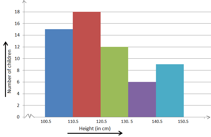
It is a perfect Presentation of the spread of numerical data. The main differentiation that separates data graphs and histograms are the gaps in the data graphs.
6. Box plots

Box plot or Box-plot is a way of representing groups of numerical data through quartiles. Data Presentation is easier with this style of graph dealing with the extraction of data to the minutes of difference.

Map Data graphs help you with data Presentation over an area to display the areas of concern. Map graphs are useful to make an exact depiction of data over a vast case scenario.
All these visual presentations share a common goal of creating meaningful insights and a platform to understand and manage the data in relation to the growth and expansion of one’s in-depth understanding of data & details to plan or execute future decisions or actions.
Importance of Data Presentation
Data Presentation could be both can be a deal maker or deal breaker based on the delivery of the content in the context of visual depiction.
Data Presentation tools are powerful communication tools that can simplify the data by making it easily understandable & readable at the same time while attracting & keeping the interest of its readers and effectively showcase large amounts of complex data in a simplified manner.
If the user can create an insightful presentation of the data in hand with the same sets of facts and figures, then the results promise to be impressive.
There have been situations where the user has had a great amount of data and vision for expansion but the presentation drowned his/her vision.
To impress the higher management and top brass of a firm, effective presentation of data is needed.
Data Presentation helps the clients or the audience to not spend time grasping the concept and the future alternatives of the business and to convince them to invest in the company & turn it profitable both for the investors & the company.
Although data presentation has a lot to offer, the following are some of the major reason behind the essence of an effective presentation:-
- Many consumers or higher authorities are interested in the interpretation of data, not the raw data itself. Therefore, after the analysis of the data, users should represent the data with a visual aspect for better understanding and knowledge.
- The user should not overwhelm the audience with a number of slides of the presentation and inject an ample amount of texts as pictures that will speak for themselves.
- Data presentation often happens in a nutshell with each department showcasing their achievements towards company growth through a graph or a histogram.
- Providing a brief description would help the user to attain attention in a small amount of time while informing the audience about the context of the presentation
- The inclusion of pictures, charts, graphs and tables in the presentation help for better understanding the potential outcomes.
- An effective presentation would allow the organization to determine the difference with the fellow organization and acknowledge its flaws. Comparison of data would assist them in decision making.
Recommended Courses

Data Visualization
Using powerbi &tableau.

Tableau for Data Analysis

MySQL Certification Program
The PowerBI Masterclass
Need help call our support team 7:00 am to 10:00 pm (ist) at (+91 999-074-8956 | 9650-308-956), keep in touch, email: [email protected].
WhatsApp us

An official website of the United States government
The .gov means it’s official. Federal government websites often end in .gov or .mil. Before sharing sensitive information, make sure you’re on a federal government site.
The site is secure. The https:// ensures that you are connecting to the official website and that any information you provide is encrypted and transmitted securely.
- Publications
- Account settings
Preview improvements coming to the PMC website in October 2024. Learn More or Try it out now .
- Advanced Search
- Journal List
- Korean J Anesthesiol
- v.70(3); 2017 Jun
Statistical data presentation
1 Department of Anesthesiology and Pain Medicine, Dongguk University Ilsan Hospital, Goyang, Korea.
Sangseok Lee
2 Department of Anesthesiology and Pain Medicine, Sanggye Paik Hospital, Inje University College of Medicine, Seoul, Korea.
Data are usually collected in a raw format and thus the inherent information is difficult to understand. Therefore, raw data need to be summarized, processed, and analyzed. However, no matter how well manipulated, the information derived from the raw data should be presented in an effective format, otherwise, it would be a great loss for both authors and readers. In this article, the techniques of data and information presentation in textual, tabular, and graphical forms are introduced. Text is the principal method for explaining findings, outlining trends, and providing contextual information. A table is best suited for representing individual information and represents both quantitative and qualitative information. A graph is a very effective visual tool as it displays data at a glance, facilitates comparison, and can reveal trends and relationships within the data such as changes over time, frequency distribution, and correlation or relative share of a whole. Text, tables, and graphs for data and information presentation are very powerful communication tools. They can make an article easy to understand, attract and sustain the interest of readers, and efficiently present large amounts of complex information. Moreover, as journal editors and reviewers glance at these presentations before reading the whole article, their importance cannot be ignored.
Introduction
Data are a set of facts, and provide a partial picture of reality. Whether data are being collected with a certain purpose or collected data are being utilized, questions regarding what information the data are conveying, how the data can be used, and what must be done to include more useful information must constantly be kept in mind.
Since most data are available to researchers in a raw format, they must be summarized, organized, and analyzed to usefully derive information from them. Furthermore, each data set needs to be presented in a certain way depending on what it is used for. Planning how the data will be presented is essential before appropriately processing raw data.
First, a question for which an answer is desired must be clearly defined. The more detailed the question is, the more detailed and clearer the results are. A broad question results in vague answers and results that are hard to interpret. In other words, a well-defined question is crucial for the data to be well-understood later. Once a detailed question is ready, the raw data must be prepared before processing. These days, data are often summarized, organized, and analyzed with statistical packages or graphics software. Data must be prepared in such a way they are properly recognized by the program being used. The present study does not discuss this data preparation process, which involves creating a data frame, creating/changing rows and columns, changing the level of a factor, categorical variable, coding, dummy variables, variable transformation, data transformation, missing value, outlier treatment, and noise removal.
We describe the roles and appropriate use of text, tables, and graphs (graphs, plots, or charts), all of which are commonly used in reports, articles, posters, and presentations. Furthermore, we discuss the issues that must be addressed when presenting various kinds of information, and effective methods of presenting data, which are the end products of research, and of emphasizing specific information.
Data Presentation
Data can be presented in one of the three ways:
–as text;
–in tabular form; or
–in graphical form.
Methods of presentation must be determined according to the data format, the method of analysis to be used, and the information to be emphasized. Inappropriately presented data fail to clearly convey information to readers and reviewers. Even when the same information is being conveyed, different methods of presentation must be employed depending on what specific information is going to be emphasized. A method of presentation must be chosen after carefully weighing the advantages and disadvantages of different methods of presentation. For easy comparison of different methods of presentation, let us look at a table ( Table 1 ) and a line graph ( Fig. 1 ) that present the same information [ 1 ]. If one wishes to compare or introduce two values at a certain time point, it is appropriate to use text or the written language. However, a table is the most appropriate when all information requires equal attention, and it allows readers to selectively look at information of their own interest. Graphs allow readers to understand the overall trend in data, and intuitively understand the comparison results between two groups. One thing to always bear in mind regardless of what method is used, however, is the simplicity of presentation.

| Variable | Group | Baseline | After drug | 1 min | 3 min | 5 min |
|---|---|---|---|---|---|---|
| SBP | C | 135.1 ± 13.4 | 139.2 ± 17.1 | 186.0 ± 26.6 | 160.1 ± 23.2 | 140.7 ± 18.3 |
| D | 135.4 ± 23.8 | 131.9 ± 13.5 | 165.2 ± 16.2 | 127.9 ± 17.5 | 108.4 ± 12.6 | |
| DBP | C | 79.7 ± 9.8 | 79.4 ± 15.8 | 104.8 ± 14.9 | 87.9 ± 15.5 | 78.9 ± 11.6 |
| D | 76.7 ± 8.3 | 78.4 ± 6.3 | 97.0 ± 14.5 | 74.1 ± 8.3 | 66.5 ± 7.2 | |
| MBP | C | 100.3 ± 11.9 | 103.5 ± 16.8 | 137.2 ± 18.3 | 116.9 ± 16.2 | 103.9 ± 13.3 |
| D | 97.7 ± 14.9 | 98.1 ± 8.7 | 123.4 ± 13.8 | 95.4 ± 11.7 | 83.4 ± 8.4 |
Values are expressed as mean ± SD. Group C: normal saline, Group D: dexmedetomidine. SBP: systolic blood pressure, DBP: diastolic blood pressure, MBP: mean blood pressure, HR: heart rate. * P < 0.05 indicates a significant increase in each group, compared with the baseline values. † P < 0.05 indicates a significant decrease noted in Group D, compared with the baseline values. ‡ P < 0.05 indicates a significant difference between the groups.
Text presentation
Text is the main method of conveying information as it is used to explain results and trends, and provide contextual information. Data are fundamentally presented in paragraphs or sentences. Text can be used to provide interpretation or emphasize certain data. If quantitative information to be conveyed consists of one or two numbers, it is more appropriate to use written language than tables or graphs. For instance, information about the incidence rates of delirium following anesthesia in 2016–2017 can be presented with the use of a few numbers: “The incidence rate of delirium following anesthesia was 11% in 2016 and 15% in 2017; no significant difference of incidence rates was found between the two years.” If this information were to be presented in a graph or a table, it would occupy an unnecessarily large space on the page, without enhancing the readers' understanding of the data. If more data are to be presented, or other information such as that regarding data trends are to be conveyed, a table or a graph would be more appropriate. By nature, data take longer to read when presented as texts and when the main text includes a long list of information, readers and reviewers may have difficulties in understanding the information.
Table presentation
Tables, which convey information that has been converted into words or numbers in rows and columns, have been used for nearly 2,000 years. Anyone with a sufficient level of literacy can easily understand the information presented in a table. Tables are the most appropriate for presenting individual information, and can present both quantitative and qualitative information. Examples of qualitative information are the level of sedation [ 2 ], statistical methods/functions [ 3 , 4 ], and intubation conditions [ 5 ].
The strength of tables is that they can accurately present information that cannot be presented with a graph. A number such as “132.145852” can be accurately expressed in a table. Another strength is that information with different units can be presented together. For instance, blood pressure, heart rate, number of drugs administered, and anesthesia time can be presented together in one table. Finally, tables are useful for summarizing and comparing quantitative information of different variables. However, the interpretation of information takes longer in tables than in graphs, and tables are not appropriate for studying data trends. Furthermore, since all data are of equal importance in a table, it is not easy to identify and selectively choose the information required.
For a general guideline for creating tables, refer to the journal submission requirements 1) .
Heat maps for better visualization of information than tables
Heat maps help to further visualize the information presented in a table by applying colors to the background of cells. By adjusting the colors or color saturation, information is conveyed in a more visible manner, and readers can quickly identify the information of interest ( Table 2 ). Software such as Excel (in Microsoft Office, Microsoft, WA, USA) have features that enable easy creation of heat maps through the options available on the “conditional formatting” menu.
| Example of a regular table | Example of a heat map | ||||||
|---|---|---|---|---|---|---|---|
| SBP | DBP | MBP | HR | SBP | DBP | MBP | HR |
| 128 | 66 | 87 | 87 | 128 | 66 | 87 | 87 |
| 125 | 43 | 70 | 85 | 125 | 43 | 70 | 85 |
| 114 | 52 | 68 | 103 | 114 | 52 | 68 | 103 |
| 111 | 44 | 66 | 79 | 111 | 44 | 66 | 79 |
| 139 | 61 | 81 | 90 | 139 | 61 | 81 | 90 |
| 103 | 44 | 61 | 96 | 103 | 44 | 61 | 96 |
| 94 | 47 | 61 | 83 | 94 | 47 | 61 | 83 |
All numbers were created by the author. SBP: systolic blood pressure, DBP: diastolic blood pressure, MBP: mean blood pressure, HR: heart rate.
Graph presentation
Whereas tables can be used for presenting all the information, graphs simplify complex information by using images and emphasizing data patterns or trends, and are useful for summarizing, explaining, or exploring quantitative data. While graphs are effective for presenting large amounts of data, they can be used in place of tables to present small sets of data. A graph format that best presents information must be chosen so that readers and reviewers can easily understand the information. In the following, we describe frequently used graph formats and the types of data that are appropriately presented with each format with examples.
Scatter plot
Scatter plots present data on the x - and y -axes and are used to investigate an association between two variables. A point represents each individual or object, and an association between two variables can be studied by analyzing patterns across multiple points. A regression line is added to a graph to determine whether the association between two variables can be explained or not. Fig. 2 illustrates correlations between pain scoring systems that are currently used (PSQ, Pain Sensitivity Questionnaire; PASS, Pain Anxiety Symptoms Scale; PCS, Pain Catastrophizing Scale) and Geop-Pain Questionnaire (GPQ) with the correlation coefficient, R, and regression line indicated on the scatter plot [ 6 ]. If multiple points exist at an identical location as in this example ( Fig. 2 ), the correlation level may not be clear. In this case, a correlation coefficient or regression line can be added to further elucidate the correlation.

Bar graph and histogram
A bar graph is used to indicate and compare values in a discrete category or group, and the frequency or other measurement parameters (i.e. mean). Depending on the number of categories, and the size or complexity of each category, bars may be created vertically or horizontally. The height (or length) of a bar represents the amount of information in a category. Bar graphs are flexible, and can be used in a grouped or subdivided bar format in cases of two or more data sets in each category. Fig. 3 is a representative example of a vertical bar graph, with the x -axis representing the length of recovery room stay and drug-treated group, and the y -axis representing the visual analog scale (VAS) score. The mean and standard deviation of the VAS scores are expressed as whiskers on the bars ( Fig. 3 ) [ 7 ].

By comparing the endpoints of bars, one can identify the largest and the smallest categories, and understand gradual differences between each category. It is advised to start the x - and y -axes from 0. Illustration of comparison results in the x - and y -axes that do not start from 0 can deceive readers' eyes and lead to overrepresentation of the results.
One form of vertical bar graph is the stacked vertical bar graph. A stack vertical bar graph is used to compare the sum of each category, and analyze parts of a category. While stacked vertical bar graphs are excellent from the aspect of visualization, they do not have a reference line, making comparison of parts of various categories challenging ( Fig. 4 ) [ 8 ].

A pie chart, which is used to represent nominal data (in other words, data classified in different categories), visually represents a distribution of categories. It is generally the most appropriate format for representing information grouped into a small number of categories. It is also used for data that have no other way of being represented aside from a table (i.e. frequency table). Fig. 5 illustrates the distribution of regular waste from operation rooms by their weight [ 8 ]. A pie chart is also commonly used to illustrate the number of votes each candidate won in an election.

Line plot with whiskers
A line plot is useful for representing time-series data such as monthly precipitation and yearly unemployment rates; in other words, it is used to study variables that are observed over time. Line graphs are especially useful for studying patterns and trends across data that include climatic influence, large changes or turning points, and are also appropriate for representing not only time-series data, but also data measured over the progression of a continuous variable such as distance. As can be seen in Fig. 1 , mean and standard deviation of systolic blood pressure are indicated for each time point, which enables readers to easily understand changes of systolic pressure over time [ 1 ]. If data are collected at a regular interval, values in between the measurements can be estimated. In a line graph, the x-axis represents the continuous variable, while the y-axis represents the scale and measurement values. It is also useful to represent multiple data sets on a single line graph to compare and analyze patterns across different data sets.
Box and whisker chart
A box and whisker chart does not make any assumptions about the underlying statistical distribution, and represents variations in samples of a population; therefore, it is appropriate for representing nonparametric data. AA box and whisker chart consists of boxes that represent interquartile range (one to three), the median and the mean of the data, and whiskers presented as lines outside of the boxes. Whiskers can be used to present the largest and smallest values in a set of data or only a part of the data (i.e. 95% of all the data). Data that are excluded from the data set are presented as individual points and are called outliers. The spacing at both ends of the box indicates dispersion in the data. The relative location of the median demonstrated within the box indicates skewness ( Fig. 6 ). The box and whisker chart provided as an example represents calculated volumes of an anesthetic, desflurane, consumed over the course of the observation period ( Fig. 7 ) [ 9 ].

Three-dimensional effects
Most of the recently introduced statistical packages and graphics software have the three-dimensional (3D) effect feature. The 3D effects can add depth and perspective to a graph. However, since they may make reading and interpreting data more difficult, they must only be used after careful consideration. The application of 3D effects on a pie chart makes distinguishing the size of each slice difficult. Even if slices are of similar sizes, slices farther from the front of the pie chart may appear smaller than the slices closer to the front ( Fig. 8 ).

Drawing a graph: example
Finally, we explain how to create a graph by using a line graph as an example ( Fig. 9 ). In Fig. 9 , the mean values of arterial pressure were randomly produced and assumed to have been measured on an hourly basis. In many graphs, the x- and y-axes meet at the zero point ( Fig. 9A ). In this case, information regarding the mean and standard deviation of mean arterial pressure measurements corresponding to t = 0 cannot be conveyed as the values overlap with the y-axis. The data can be clearly exposed by separating the zero point ( Fig. 9B ). In Fig. 9B , the mean and standard deviation of different groups overlap and cannot be clearly distinguished from each other. Separating the data sets and presenting standard deviations in a single direction prevents overlapping and, therefore, reduces the visual inconvenience. Doing so also reduces the excessive number of ticks on the y-axis, increasing the legibility of the graph ( Fig. 9C ). In the last graph, different shapes were used for the lines connecting different time points to further allow the data to be distinguished, and the y-axis was shortened to get rid of the unnecessary empty space present in the previous graphs ( Fig. 9D ). A graph can be made easier to interpret by assigning each group to a different color, changing the shape of a point, or including graphs of different formats [ 10 ]. The use of random settings for the scale in a graph may lead to inappropriate presentation or presentation of data that can deceive readers' eyes ( Fig. 10 ).

Owing to the lack of space, we could not discuss all types of graphs, but have focused on describing graphs that are frequently used in scholarly articles. We have summarized the commonly used types of graphs according to the method of data analysis in Table 3 . For general guidelines on graph designs, please refer to the journal submission requirements 2) .
| Analysis | Subgroup | Number of variables | Type |
|---|---|---|---|
| Comparison | Among items | Two per items | Variable width column chart |
| One per item | Bar/column chart | ||
| Over time | Many periods | Circular area/line chart | |
| Few periods | Column/line chart | ||
| Relationship | Two | Scatter chart | |
| Three | Bubble chart | ||
| Distribution | Single | Column/line histogram | |
| Two | Scatter chart | ||
| Three | Three-dimensional area chart | ||
| Comparison | Changing over time | Only relative differences matter | Stacked 100% column chart |
| Relative and absolute differences matter | Stacked column chart | ||
| Static | Simple share of total | Pie chart | |
| Accumulation | Waterfall chart | ||
| Components of components | Stacked 100% column chart with subcomponents |
Conclusions
Text, tables, and graphs are effective communication media that present and convey data and information. They aid readers in understanding the content of research, sustain their interest, and effectively present large quantities of complex information. As journal editors and reviewers will scan through these presentations before reading the entire text, their importance cannot be disregarded. For this reason, authors must pay as close attention to selecting appropriate methods of data presentation as when they were collecting data of good quality and analyzing them. In addition, having a well-established understanding of different methods of data presentation and their appropriate use will enable one to develop the ability to recognize and interpret inappropriately presented data or data presented in such a way that it deceives readers' eyes [ 11 ].
<Appendix>
Output for presentation.
Discovery and communication are the two objectives of data visualization. In the discovery phase, various types of graphs must be tried to understand the rough and overall information the data are conveying. The communication phase is focused on presenting the discovered information in a summarized form. During this phase, it is necessary to polish images including graphs, pictures, and videos, and consider the fact that the images may look different when printed than how appear on a computer screen. In this appendix, we discuss important concepts that one must be familiar with to print graphs appropriately.
The KJA asks that pictures and images meet the following requirement before submission 3)
“Figures and photographs should be submitted as ‘TIFF’ files. Submit files of figures and photographs separately from the text of the paper. Width of figure should be 84 mm (one column). Contrast of photos or graphs should be at least 600 dpi. Contrast of line drawings should be at least 1,200 dpi. The Powerpoint file (ppt, pptx) is also acceptable.”
Unfortunately, without sufficient knowledge of computer graphics, it is not easy to understand the submission requirement above. Therefore, it is necessary to develop an understanding of image resolution, image format (bitmap and vector images), and the corresponding file specifications.
Resolution is often mentioned to describe the quality of images containing graphs or CT/MRI scans, and video files. The higher the resolution, the clearer and closer to reality the image is, while the opposite is true for low resolutions. The most representative unit used to describe a resolution is “dpi” (dots per inch): this literally translates to the number of dots required to constitute 1 inch. The greater the number of dots, the higher the resolution. The KJA submission requirements recommend 600 dpi for images, and 1,200 dpi 4) for graphs. In other words, resolutions in which 600 or 1,200 dots constitute one inch are required for submission.
There are requirements for the horizontal length of an image in addition to the resolution requirements. While there are no requirements for the vertical length of an image, it must not exceed the vertical length of a page. The width of a column on one side of a printed page is 84 mm, or 3.3 inches (84/25.4 mm ≒ 3.3 inches). Therefore, a graph must have a resolution in which 1,200 dots constitute 1 inch, and have a width of 3.3 inches.
Bitmap and Vector
Methods of image construction are important. Bitmap images can be considered as images drawn on section paper. Enlarging the image will enlarge the picture along with the grid, resulting in a lower resolution; in other words, aliasing occurs. On the other hand, reducing the size of the image will reduce the size of the picture, while increasing the resolution. In other words, resolution and the size of an image are inversely proportionate to one another in bitmap images, and it is a drawback of bitmap images that resolution must be considered when adjusting the size of an image. To enlarge an image while maintaining the same resolution, the size and resolution of the image must be determined before saving the image. An image that has already been created cannot avoid changes to its resolution according to changes in size. Enlarging an image while maintaining the same resolution will increase the number of horizontal and vertical dots, ultimately increasing the number of pixels 5) of the image, and the file size. In other words, the file size of a bitmap image is affected by the size and resolution of the image (file extensions include JPG [JPEG] 6) , PNG 7) , GIF 8) , and TIF [TIFF] 9) . To avoid this complexity, the width of an image can be set to 4 inches and its resolution to 900 dpi to satisfy the submission requirements of most journals [ 12 ].
Vector images overcome the shortcomings of bitmap images. Vector images are created based on mathematical operations of line segments and areas between different points, and are not affected by aliasing or pixelation. Furthermore, they result in a smaller file size that is not affected by the size of the image. They are commonly used for drawings and illustrations (file extensions include EPS 10) , CGM 11) , and SVG 12) ).
Finally, the PDF 13) is a file format developed by Adobe Systems (Adobe Systems, CA, USA) for electronic documents, and can contain general documents, text, drawings, images, and fonts. They can also contain bitmap and vector images. While vector images are used by researchers when working in Powerpoint, they are saved as 960 × 720 dots when saved in TIFF format in Powerpoint. This results in a resolution that is inappropriate for printing on a paper medium. To save high-resolution bitmap images, the image must be saved as a PDF file instead of a TIFF, and the saved PDF file must be imported into an imaging processing program such as Photoshop™(Adobe Systems, CA, USA) to be saved in TIFF format [ 12 ].
1) Instructions to authors in KJA; section 5-(9) Table; https://ekja.org/index.php?body=instruction
2) Instructions to Authors in KJA; section 6-1)-(10) Figures and illustrations in Manuscript preparation; https://ekja.org/index.php?body=instruction
3) Instructions to Authors in KJA; section 6-1)-(10) Figures and illustrations in Manuscript preparation; https://ekja.org/index.php?body=instruction
4) Resolution; in KJA, it is represented by “contrast.”
5) Pixel is a minimum unit of an image and contains information of a dot and color. It is derived by multiplying the number of vertical and horizontal dots regardless of image size. For example, Full High Definition (FHD) monitor has 1920 × 1080 dots ≒ 2.07 million pixel.
6) Joint Photographic Experts Group.
7) Portable Network Graphics.
8) Graphics Interchange Format
9) Tagged Image File Format; TIFF
10) Encapsulated PostScript.
11) Computer Graphics Metafile.
12) Scalable Vector Graphics.
13) Portable Document Format.
We use cookies
This website uses cookies to provide better user experience and user's session management. By continuing visiting this website you consent the use of these cookies.
ChartExpo Survey

Top 5 Easy-to-Follow Data Presentation Examples
You’ll agree when we say that poring through numbers is tedious at best and mentally exhausting at worst.
And this is where data presentation examples come in.

Charts come in and distill data into meaningful insights. And this saves tons of hours, which you can use to relax or execute other tasks. Besides, when creating data stories, you need charts that communicate insights with clarity.
There are 5 solid and reliable data presentation methods: textual, statistical data presentation, measures of dispersion, tabular, and graphical data representation.
Besides, some of the tested and proven charts for data presentation include:
- Waterfall Chart
- Double Bar Graph
- Slope Chart
- Treemap Charts
- Radar Chart
- Sankey Chart
There are visualization tools that produce simple, insightful, and ready-made data presentation charts. Yes, you read that right. These tools create charts that complement data stories seamlessly.
Remember, without visualizing data to extract insights, the chances of creating a compelling narrative will go down.
Table of Content:
What is data presentation, top 5 data presentation examples:, how to generate sankey chart in excel for data presentation, importance of data presentation in business, benefits of data presentation, what are the top 5 methods of data presentation.
Data presentation is the process of using charts and graphs formats to display insights into data. The insights could be:
- Relationship
- Trend and patterns
Data Analysis and Data Presentation have a practical implementation in every possible field. It can range from academic studies, and commercial, industrial , and marketing activities to professional practices .
In its raw form, data can be extremely complicated to decipher. Examples of data presentation, such as chord diagrams , are an important step toward breaking down data into understandable charts or graphs.
You can use tools (which we’ll talk about later) to analyze raw data.
Once the required information is obtained from the data, the next logical step is to present it in a graphical presentation, such as a Box and Whisker presentation .
The presentation is the key to success.
Once you’ve extracted actionable insights, you can craft a compelling data story. Keep reading because we’ll address the following in the coming section: the importance of data presentation in business, including how tools like a Sunburst Chart can enhance your analysis.
Let’s take a look at the five data presentation examples below:
1. Waterfall Chart
A Waterfall Chart is a graphical representation used to depict the cumulative impact of sequential positive or negative values on a starting point over a designated time frame. It typically consists of a series of horizontal bars, with each bar representing a stage or category in a process.

2. Double Bar Graph

A Double Bar Chart displays more than one data series in clustered horizontal columns, similar to a clustered stacked bar chart . Each data series shares the same axis labels, so horizontal bars are grouped by category.
This arrangement allows for direct comparison of multiple series within a given category. The chart is amazingly easy to read and interpret, even for a non-technical audience.
3. Slope Chart
Slope Charts are simple graphs that quickly and directly show transitions, changes over time, absolute values, and even rankings .

Besides, they’re also called Slope Graphs .
This is one of the data presentation examples you can use to show the before and after story of variables in your data.
Slope Graphs can be useful when you have two time periods or points of comparison and want to show relative increases and decreases quickly across various categories between two data points.
A TreeMap is a data structure that stores key-value pairs in a sorted order using a Red-Black tree, ensuring efficient search, insertion, and deletion operations.
Take a look at the table below. Can you provide coherent and actionable insights into the table below?
| Macy’s-Store | Garments | Sweater | 65 |
| Macy’s-Store | Garments | Dress | 30 |
| Macy’s-Store | Garments | Hoodies | 40 |
| Macy’s-Store | Home Appliances | Refrigerator | 60 |
| Macy’s-Store | Home Appliances | Freezer | 65 |
| Macy’s-Store | Home Appliances | Oven | 70 |
| Macy’s-Store | Grocery | Fruits | 70 |
| Macy’s-Store | Grocery | Vegetables | 50 |
| Macy’s-Store | Grocery | Frozen Foods | 95 |
| Saks-Store | Garments | Sweater | 75 |
| Saks-Store | Garments | Dress | 55 |
| Saks-Store | Garments | Hoodies | 85 |
| Saks-Store | Home Appliances | Refrigerator | 65 |
| Saks-Store | Home Appliances | Freezer | 40 |
| Saks-Store | Home Appliances | Oven | 55 |
| Saks-Store | Grocery | Fruits | 45 |
| Saks-Store | Grocery | Vegetables | 85 |
| Saks-Store | Grocery | Frozen Foods | 75 |
| Belk-Store | Garments | Sweater | 95 |
| Belk-Store | Garments | Dress | 85 |
| Belk-Store | Garments | Hoodies | 65 |
| Belk-Store | Home Appliances | Refrigerator | 70 |
| Belk-Store | Home Appliances | Freezer | 55 |
| Belk-Store | Home Appliances | Oven | 95 |
| Belk-Store | Grocery | Fruits | 70 |
| Belk-Store | Grocery | Vegetables | 45 |
| Belk-Store | Grocery | Frozen Foods | 50 |
Notice the difference after visualizing the table. You can easily tell the performance of individual segments in:
- Macy’s Store

5. Radar Chart
Radar Chart is also known as Spider Chart or Spider Web Chart. A radar chart is very helpful to visualize the comparison between multiple categories and variables.

A radar Chart is one of the data presentation examples you can use to compare data of two different time ranges e.g. Current vs Previous. Radar Chart with different scales makes it easy for you to identify trends, patterns, and outliers in your data. You can also use Radar Chart to visualize the data of Polar graph equations.
6. Sankey Chart

You can use the Sankey Chart to visualize data with flow-like attributes, such as material, energy, cost, etc.
This chart draws the reader’s attention to the enormous flows, the largest consumer, the major losses , and other insights.
The aforementioned visualization design, including the Mosaic plot presentation , is one of the data presentation examples that use links and nodes to uncover hidden insights into relationships between critical metrics.
The size of a node is directly proportionate to the quantity of the data point under review.
So how can you access the data presentation examples (highlighted above)?
Excel is one of the most used tools for visualizing data because it’s easy to use.
However, you cannot access ready-made and visually appealing data presentation charts, such as a funnel chart , for storytelling. But this does not mean you should ditch this freemium data visualization tool .
Did you know you can supercharge your Excel with add-ins to access visually stunning and ready-to-go data presentation charts?
Yes, you can increase the functionality of your Excel and access ready-made data presentation examples for your data stories.
The add-on we recommend you to use is ChartExpo.
What is ChartExpo?
We recommend this tool (ChartExpo) because it’s super easy to use.
You don’t need to take programming night classes to extract insights from your data. ChartExpo is more of a ‘drag-and-drop tool,’ which means you’ll only need to scroll your mouse and fill in respective metrics and dimensions in your data, whether you’re working with Mekko presentation or other visualizations.
ChartExpo comes with a 7-day free trial period.
The tool produces charts that are incredibly easy to read and interpret . And it allows you to save charts in the world’s most recognized formats, namely PNG and JPG.
In the coming section, we’ll show you how to use ChartExpo to visualize your data with one of the data presentation examples (Sankey).
To install ChartExpo add-in into your Excel, click this link .
- Open your Excel and paste the table above.
- Click the My Apps button.

- Then select ChartExpo and click on INSERT, as shown below.

- Click the Search Box and type “Sankey Chart” .

- Once the chart pops up, click on its icon to get started.

- Select the sheet holding your data and click the Create Chart from Selection button.

How to Edit the Sankey Chart?
- Click the Edit Chart button, as shown above.

- Once the Chart Header Properties window shows, click the Line 1 box and fill in your title.

- To change the color of the nodes, click the pen-like icons on the nodes.
- Once the color window shows, select the Node Color and then the Apply button.

- Save your changes by clicking the Apply button.
- Check out the final chart below.

Data presentation examples are vital, especially when crafting data stories for the top management. Top management can use data presentation charts, such as Sankey, as a backdrop for their decision.
Presentation charts, maps, and graphs are powerful because they simplify data by making it understandable & readable at the same time. Besides, they make data stories compelling and irresistible to target audiences.
Big files with numbers are usually hard to read and make it difficult to spot patterns easily. However, many businesses believe that developing visual reports focused on creating stories around data is unnecessary; they think that the data alone should be sufficient for decision-making.
Visualizing supports this and lightens the decision-making process.
Luckily, there are innovative applications you can use to visualize all the data your company has into dashboards, graphs, and reports. Data visualization helps transform your numbers into an engaging story with details and patterns.
Check out more benefits of data presentation examples below:
1. Easy to understand
You can interpret vast quantities of data clearly and cohesively to draw insights, thanks to graphic representations.
Using data presentation examples, such as charts, managers and decision-makers can easily create and rapidly consume key metrics.
If any of the aforementioned metrics have anomalies — ie. sales are significantly down in one region — decision-makers will easily dig into the data to diagnose the problem.
2. Spot patterns
Data visualization can help you to do trend analysis and respond rapidly on the grounds of what you see.
Such patterns make more sense when graphically represented; because charts make it easier to identify correlated parameters.
3. Data Narratives
You can use data presentation charts, such as Sankey or Area Charts , to build dashboards and turn them into stories.
Data storytelling can help you connect with potential readers and audiences on an emotional level.
4. Speed up the decision-making process
We naturally process visual images 60,000 times faster than text. A graph, chart, or other visual representation of data is more comfortable for our brain to process.
Thanks to our ability to easily interpret visual content, data presentation examples can dramatically improve the speed of decision-making processes.
Take a look at the table below.
| Pouches | 70 | 100 |
| Holsters | 50 | 85 |
| Shells | 80 | 60 |
| Skins | 100 | 120 |
| Fitted cases | 70 | 60 |
| Bumpers | 65 | 80 |
| Flip cases | 90 | 100 |
| Sleeves | 50 | 45 |
Can you give reliable insights into the table above?
Keep reading because we’ll explore easy-to-follow data presentation examples in the coming section. Also, we’ll address the following question: what are the top 5 methods of data presentation?
1. Textual Ways of Presenting Data
Out of the five data presentation examples, this is the simplest one.
Just write your findings coherently and your job is done. The demerit of this method is that one has to read the whole text to get a clear picture. Yes, you read that right.
The introduction, summary, and conclusion can help condense the information.
2. Statistical data presentation
Data on its own is less valuable. However, for it to be valuable to your business, it has to be:
No matter how well manipulated, the insights into raw data should be presented in an easy-to-follow sequence to keep the audience waiting for more.
Text is the principal method for explaining findings, outlining trends, and providing contextual information. A table is best suited for representing individual information and represents both quantitative and qualitative information.
On the other hand, a graph is a very effective visual tool because:
- It displays data at a glance
- Facilitates comparison
- Reveals trends, relationships, frequency distribution, and correlation
Text, tables, and graphs are incredibly effective data presentation examples you can leverage to curate persuasive data narratives.
3. Measure of Dispersion
Statistical dispersion is how a key metric is likely to deviate from the average value. In other words, dispersion can help you to understand the distribution of key data points.
There are two types of measures of dispersion, namely:
- Absolute Measure of Dispersion
- Relative Measure of Dispersion
4. Tabular Ways of Data Presentation and Analysis
To avoid the complexities associated with qualitative data, use tables and charts to display insights.
This is one of the data presentation examples where values are displayed in rows and columns. All rows and columns have an attribute (name, year, gender, and age).
5. Graphical Data Representation
Graphical representation uses charts and graphs to visually display, analyze, clarify, and interpret numerical data, functions, and other qualitative structures.
Data is ingested into charts and graphs, such as Sankey, and then represented by a variety of symbols, such as lines and bars.
Data presentation examples, such as Bar Charts , can help you illustrate trends, relationships, comparisons, and outliers between data points.
What is the main objective of data presentation?
Discovery and communication are the two key objectives of data presentation.
In the discovery phase, we recommend you try various charts and graphs to understand the insights into the raw data. The communication phase is focused on presenting the insights in a summarized form.
What is the importance of graphs and charts in business?
Big files with numbers are usually hard to read and make it difficult to spot patterns easily.
Presentation charts, maps, and graphs are vital because they simplify data by making it understandable & readable at the same time. Besides, they make data stories compelling and irresistible to target audiences.
Poring through numbers is tedious at best and mentally exhausting at worst.
This is where data presentation examples come into play.
Charts come in and distill data into meaningful insights. And this saves tons of hours, which you can use to handle other tasks. Besides, when creating data stories, it would be best if you had charts that communicate insights with clarity.
Excel, one of the popular tools for visualizing data, comes with very basic data presentation charts, which require a lot of editing.
We recommend you try ChartExpo because it’s one of the most trusted add-ins. Besides, it has a super-friendly user interface for everyone, irrespective of their computer skills.
Create simple, ready-made, and easy-to-interpret Bar Charts today without breaking a sweat.
How much did you enjoy this article?

Related articles
Balanced Scorecard: What is It, Uses, & Implementation
Explore Balanced Scorecard's role in aligning organizational activities with strategic goals, enhancing decision-making, and measuring performance effectively.
Breast Cancer Charts for Clear and Effective Insights
Discover the importance of Breast Cancer Charts in visualizing trends and statistics, helping in effective communication & analysis of breast cancer information.
Hemoglobin A1C: What It is, Test, and Chart
Unlock the power of Hemoglobin A1C Chart to track and improve your diabetes management with expert insights & detailed analysis for better health outcomes.
Time Series Analysis: What is it, Types and Best Practices
What is Time Series Data? Discover its importance in analyzing trends. Explore types, & best practices for using this data in fields like finance, and healthcare.
How to Create a Report in Excel: A Complete Guide
Learn how to create a report in Excel and elevate your analysis capabilities. This guide will walk you through the process of turning data into actionable insights.
Presentation of Data
Data can be represented in countless ways. The format for the presentation of data will depend on the target audience and the information that needs to be relayed. In the end, data should be presented in such a way that interpretation and analysis is made easy. Let us see some ways in which we represent data in economics.
- Diagrammatic Presentation of Data
- Textual and Tabular Presentation of Data
Customize your course in 30 seconds
- Accountancy
- Business Studies
- Organisational Behaviour
- Human Resource Management
- Entrepreneurship
Textual Presentation of Data: Meaning, Suitability, and Drawbacks
Presentation of Data refers to the exhibition of data in such a clear and attractive way that it is easily understood and analysed. Data can be presented in different forms, including Textual or Descriptive Presentation, Tabular Presentation, and Diagrammatic Presentation.
Textual Presentation
Textual or Descriptive Presentation of Data is one of the most common forms of data presentation. In this, data is a part of the text of the study or a part of the description of the subject matter of the study. It is usually preferred when the quantity of data is not very large. For example, there are 50 students in a class, among them 30 are boys and 20 are girls. This is the data that can be understood with the help of a simple text and no table or pie diagram is required for the same.

Suitability
Textual Presentation of Data is suitable when the quantity of data is not large. It means that a small portion of data that is presented as a part of the subject matter of study can become useful supportive evidence to the given text. Therefore, instead of saying that the price of petrol is skyrocketing, it can be said that the price of petrol has increased by 20% in the last 2 years, and this statement will be more meaningful and precise. Under textual presentation of data, an individual does not have to support the text with the help of a diagram or table as the text in itself is very small and has few observations.
Advantages of Textual Presentation of Data
Textual Presentation of Data has the following benefits:
1. It allows the researcher to make an elaborate interpretation of data during the presentation.
2. A researcher can easily present qualitative data that cannot be presented in tabular or graphical form using the textual presentation of data.
3. If the data is present in small sets, a textual presentation can be easily used. For example, there are 50 students in a class, among them, 30 are boys and 20 are girls. This is the data that can be understood with the help of a simple text and no table or pie diagram is required for the same.
Disadvantages of Textual Presentation of Data
Textual Presentation of Data has the following drawbacks:
1. One of the major drawbacks of the textual presentation of data is that it provides extensive data in the form of text and paragraphs which makes it difficult for the user of data to draw a proper conclusion at a glance. This facility is provided in tabular or diagrammatic presentation of data.
2. This method of presenting data is not suitable for large sets of data as these sets contain too many details.
3. Besides, one has to read through the whole text in order to understand and comprehend the main point of the data.
Please Login to comment...
Similar reads.
- Statistics for Economics
- Commerce - 11th
- How to Get a Free SSL Certificate
- Best SSL Certificates Provider in India
- Elon Musk's xAI releases Grok-2 AI assistant
- What is OpenAI SearchGPT? How it works and How to Get it?
- Content Improvement League 2024: From Good To A Great Article
Improve your Coding Skills with Practice
What kind of Experience do you want to share?
- Meet Our Team
- Learn | Download App
TEXTUAL, TABULAR & DIAGRAMMATIC PRESENTATION OF DATA

STATISTICS : PRESENTATION OF DATA
Data can be presented in three ways:
- Textual presentation
- Tabular presentation
- Diagrammatic presentation
1. Textual Mode of presentation is layman’s method of presentation of data. Anyone can prepare, anyone can understand. No specific skill(s) is/are required.
2. Tabular Mode of presentation is the most accurate mode of presentation of data. It requires a lot of skill to prepare, and some skill(s) to understand. Table facilitates comparison.
But, Table should be good enough as per some points of view:
- 1. Appealing
- 2. Well-balanced
- 3. Compulsory Title and Table Number
- 4. Title should be self-explanatory
- 5. Units must be properly mentioned
- 6. Comparison should be easy
- 7. Sources and footnotes (if any) must be mentioned at the bottom
Below is a sample of how a table should look like:
Table No. 1: Format of a table
| CAPTION | ||
Height (cm) | Weight (kg) | Age (Years) | |
STUB |
BODY OF THE TABLE
| ||
* Sources: 1. Kailasha Foundation – Fun & Learn Portal LMS Directory *Footnotes: The entire upper part of the table is called BOX HEAD.
3. Diagrammatic Mode of Presentation:
A. Non-Frequency Diagrams: Non-frequency diagrams correspond to the data which are NOT frequency data. (a) Bar Diagrams (b) Line Diagrams (Historiagram) (c) Pie Diagram or Pie Chart
B. Frequency Diagrams: Frequency Data are presented. Mostly class-intervals are presented via this mode. Three most common frequency diagrams are: (a) Histogram (b) Frequency Polygon (c) Ogives: (i) Less than type Ogives (ii) More than type Ogives
- 1. Bar Diagram and Line Diagram are inter-convertible
- 2. Bar Diagram and Line Diagram can both be of simple and multiple types
- 3. Multiple bar diagram or Multiple Line diagram is used when two related series (in same unit) are to be compared
- 4. Multiple axis bar diagram or Multiple axis Line diagram is used when units in the two series are different
ILLUSTRATIONS OF PRESENTATION OF DATA:
Bar Diagrams:
Line Diagram:

Multiple Bar Diagram:

Frequency Polygon:

FREQUENCY CURVE:
A smooth join of all vertices of a frequency polygon. This is broadly divided into four shapes:
(i) Bell Shaped (Most Common Shape) (ii) U-Shaped (iii) J – Shaped: Simple J – shaped & Inverted J – Shaped (iv) Mixed Curve (Second Most Common Shape)
- 1. CENSUS: The collection of data from every element in a population or universe or arena of statistical enquiry.
- 2. SAMPLE: The collection of data from subgroup or subset of the population.
- 3. FREQUENCY: The number of times a certain value or class of values occurs.
- 4. CUMULATIVE FREQUENCY: The running total of the frequencies at each class interval level.
- 5. FREQUENCY DISTRIBUTION: The organization of raw data in table form with classes and frequencies.
- 6. CLASS LIMITS: The originally assigned extreme values of classes are called class limits, viz. Lower class limit and upper class limit.
- 7. CLASS WIDTH: The difference between the upper and lower boundaries (NOT limits) of any class.
- 8. CLASS BOUNDARY: After making the distribution continuous, the upper class boundary of a class becomes equal to the lower class boundary of the next class.
- 9. CLASS MARK: The mid-point of any class is called the class mark.
VIDEO DESCRIPTIONS:
Hindi explanation:.
ENGLISH EXPLANATION:
Thanks for learning at Kailasha Foundation – Fun & Learn Portal.
Share this course with friends. Follow us on Facebook , twitter to stay updated.
Related Posts

Become an actuary to step out of the crowd

NOUNS – Lecture 1

Leave a Reply Cancel reply
This site uses Akismet to reduce spam. Learn how your comment data is processed .
Thank you for visiting nature.com. You are using a browser version with limited support for CSS. To obtain the best experience, we recommend you use a more up to date browser (or turn off compatibility mode in Internet Explorer). In the meantime, to ensure continued support, we are displaying the site without styles and JavaScript.
- View all journals
- Explore content
- About the journal
- Publish with us
- Sign up for alerts
- Open access
- Published: 26 August 2024
Quantification of the time-varying epidemic growth rate and of the delays between symptom onset and presenting to healthcare for the mpox epidemic in the UK in 2022
- Robert Hinch 1 na1 ,
- Jasmina Panovska-Griffiths 1 , 2 , 3 na1 ,
- Thomas Ward 3 ,
- Andre Charlett 3 ,
- Nicholas Watkins 3 &
- Christophe Fraser 1
Scientific Reports volume 14 , Article number: 19755 ( 2024 ) Cite this article
Metrics details
- Infectious diseases
The mpox epidemic in the UK began in May 2022, with rates of new cases unexpectedly and rapidly declining during August 2022. Interpreting trends in infection requires disentangling the underlying growth rate of cases from the delay from symptom onset to presenting to healthcare. We developed a nowcasting Bayesian method which incorporates time-varying delays (EpiLine) to quantify the changes in the delay from symptom onset to healthcare presentation and the underlying mpox growth rate over the period May-August 2022 in the UK. We show that the mean delay between symptom onset and healthcare presentation for mpox in the UK decreased from 22 days in early May 2022 to 10 days by early June and 8 days in August 2022. When we account for these dynamic delays, the time-varying growth rate declined gradually and continuously in the UK during the May-August 2022 period. Not accounting for varying time delays would have incorrectly characterised the growth rate by a sharp increase followed by a rapid decline in mpox cases. Our results highlight the importance of correctly quantifying the delay between symptom onset to healthcare presentation when characterising the epidemic growth of mpox in the UK. The gradual reduction in the rate of epidemic spread, which pre-dated the vaccine roll-out, is consistent with gradual risk reduction or acquired immunity amongst the highest risk individuals. Our study highlights the need for public health agencies to record the delays from symptom onset to healthcare presentation early in an outbreak.
Introduction
Mpox (monkeypox) is a zoonotic infection caused by a virus that belongs to the family of Orthopoxvirus. Since the first human reported case of mpox in the Democratic Republic of Congo in 1970, sporadic human cases have been identified both inside and outside of Africa 1 . On May 7, 2022, mpox was detected in a traveller returning to the United Kingdom from Nigeria, with the rate of reported cases in the UK then increasing until mid-July before declining (Fig. 1 a) 2 .

Estimated reporting delay and epidemic growth rate \(r\left( t \right)\) using UKHSA data. ( a ) Number of daily reported cases and daily symptoms onset (only reported by 40–80% cases) along with the fitted posterior density of the symptoms onset (for all reported cases). For the vast majority of reported cases in May the symptoms onset date is known, thus the posterior distribution and the reported data fit well to mid-May. For cases reported from June onwards, the proportion for which the date of symptoms onset was known declined, thus the reported symptoms onset is less than the posterior distribution. ( b ) Distribution of the reported delays (the time between onset of symptoms and reporting to healthcare providers) for those developing symptoms at the start of May and June 2022. ( c ) Epidemic growth rate \(r\left( t \right)\) of mpox in the UK when accounting for dynamic reporting delays, showing a gradual decline over the reporting period. The right-axis converts \(r\left( t \right)\) to a doubling or halving time. ( d ) Estimates (median and 25,75 percentiles) of the reported delay indexed by the date of symptoms onset. In all graphs the solid lines are the median estimates and the shaded area being the 5%-95% confidence interval.
Mpox virus is an infectious pathogen which can be transmitted through close physical contact and fomites. Since the onset of the mpox epidemic in the UK in early May 2022, and over the epidemic period May–September 2022, the UK Health Security Agency (UKHSA) has been monitoring and responding to the outbreak in the UK 8 . As part of the response, our group had access to mpox data and tracked the epidemic potential giving informed advice to aid public health policy.
During the 2022 outbreak, mpox cases were predominantly amongst gay and bisexual men who have sex with men (GBMSM) with clusters of cases linked with venues where individuals were exposed to the virus through close, often sexual, contact 3 . Pre-symptomatic transmission was found to be a significant component of this outbreak, with approximately 53% of transmission prior to symptom onset 4 . Initial symptoms for mpox can be influenza-like (e.g. fever or sore throat) with reported incubation periods of 3–20 days 5 and mean incubation period of 7–9 days 5 , 6 . This is followed by smallpox-like rashes, which sequentially progress to macules, papules and vesicles before crusting over after 2–4 weeks 7 . Within the UK mpox epidemic, healthcare professionals obtained details of symptoms and their time of onset for a fraction of the confirmed cases. There was a variation in the uncertainty around the date-dependant confirmed cases from 77/97 confirmed cases (~ 80%) in the first two weeks of the outbreak in May 2022 to 163/495 confirmed cases (~ 40%) during August 2022 8 . Initially, the delay between the onset of symptoms and presenting to healthcare providers was up to a month (based on data within UKHSA mpox response group). As the awareness of the disease increases, due to public health information or other interventions, the delays in presenting to healthcare providers may decrease with people reporting infection earlier.
When models are fit to epidemics, one would ideally have data on the number of people infected each day. However, the data typically available is the number of symptomatic cases who present to healthcare providers each day (i.e. reported cases). Therefore, models are normally fit to the reported cases, with the delay between infection and reporting being modelled as a static distribution. This delay distribution consists of the incubation period (infection to symptoms) and the delay from symptom onset to accessing healthcare, and is typically estimated from detailed studies on a subset of early cases in the epidemic. Whilst the incubation period is not expected to change over time, the delay between symptom onset and accessing healthcare is likely to decrease as public awareness of the epidemic increases. If this delay from symptom onset to healthcare presentation decreases rapidly, it would lead to a surge in reported cases due to the effect of people at different stages of disease presenting to healthcare providers at the same time. Hence it is important to quantify how the time between symptom onset and healthcare presentation changes in the course of an epidemic.
The general approach in modelling mpox 2022 epidemic was either using Bayesian models such as 20 or a more mechanistic SEIR model 11 that allow for processes such as vaccination to be more readily modelled. The former model used Bayesian doubly interval censored model adjusted for right truncation to calculate the time from infection to hospital admission, infection to a first positive test, and the length of hospital stay whilst keeping the distribution of infection to symptom onset uniform. The latter model had constant time from symptom onset to presenting to healthcare and focused on evaluating the impact of vaccination on the trajectory of the mpox epidemic.
The two aims of our study were to quantify time-varying delays between symptom onset and healthcare presentation, and also the time-varying epidemic growth rate of the mpox epidemic in the UK in 2022. This is non-trivial since both together contribute to observed data, and so require statistical deconvolution (disentangling). The two datasets we used were the total number of reported cases, and the self-reported symptoms onset time which was provided by a subset of cases. At the time of analysis, we did not find required statistical tools within existing ‘nowcasting’ software, and so to perform this analysis, we developed a Bayesian model (“EpiLine”) which simultaneously estimated the time-varying delay between symptom onset and healthcare presentation and the epidemic growth rate over the period May–August 2022 in the UK.
In this study, we illustrate the development and application of a custom nowcasting Bayesian method which incorporates time-varying delays (EpiLine) to simulate the growth rate of symptomatic cases, from both actual mpox data in the UK as well as simulated data, aiming to quantify the time between mpox symptom onset to healthcare presentation and the growth rate over the mpox epidemic in the UK in 2022.
EpiLine model
To jointly quantify the changes in delays in the distribution of time \(\tau\) from symptom onset to healthcare presentation at time \(t\) , denoted \(f\left( {\tau ,t - \tau } \right)\) and its effect on estimating the epidemic growth rate, denoted \(r\left( t \right)\) . We developed a Bayesian model incorporating both a dynamic growth rate and dynamic delays called EpiLine ( https://github.com/BDI-pathogens/EpiLine ). The model was implemented in R software ( https://www.r-project.org ), version 4.1.3.
The model was built to understand the interaction between the symptom-healthcare presentation time distribution and the underlying dynamics of the infection rate, therefore we use a very simple model for the number of people developing the symptoms each day. The model contains a generative model which calculates the expected number of reported cases on a particular day, and an observation model for the observed data (same approach as Epidemia uses for estimating daily deaths 19 ). We model the daily growth rate \(r\left( t \right)\) with a simple Gaussian process, the daily number of people of developing symptoms \(S\left( t \right)\) is given by
where \(\sigma_{rGP}^{2}\) is the daily variance of the Gaussian process. Gaussian processes were used because of their flexibility to model time varying processes and provide confidence intervals even when the underlying mechanisms for time variation are unknown. Note that by making \(r\left( t \right)\) a Gaussian process instead of \(S\left( t \right)\) implies the prior is that the change in \(S\left( t \right)\) is the same as the previous day. Next we define \(f\left( {\tau ,t} \right)\) as the probability of someone presenting to healthcare with an infection on day \((t + \tau\) ), if they developed symptoms on day \(t\) . Note that \(\tau\) can be negative if a case is found prior to symptoms developing (e.g. if contact-traced and tested positive). On day \(t\) the expected number of cases presenting to healthcare is \(\mu \left( t \right)\) and given by
where \(\tau_{pre}\) is the maximum number of days pre-reporting the case develops symptoms and \(\tau_{post}\) the maximum number of days post-reporting the case develops symptoms. The number of observed cases presenting to healthcare \(C\left( t \right)\) is modelled as a negative binomial variable
where \(\phi_{OD}\) is the over-dispersion parameter. The symptom-healthcare presentation time distribution must support both positive and negative values. In addition, empirically it is observed that this distribution can be highly skewed with heavy tails, therefore we model it using the Johnson SU distribution which contains four parameters \((\xi ,\lambda ,\gamma ,\delta\) , so can fit mean, variance, skew and kurtosis). To account for the changes in the distribution over time, we model these four parameters using simple Gaussian processes
At the end of the reporting period, there may not be many cases presenting to healthcare for each symptoms date (since the data is right censored), therefore there is the option to make the distribution static after a particular time \(t_{static}\) (i.e. when then \(t > t_{static}\) \(\xi \left( t \right) = \xi \left( {t_{static} } \right)).\) These parameters are estimated using line list data of individual cases where the symptoms date and healthcare presentation date are known. Note, cases where only the healthcare presentation date is known are included in the daily report totals \(C\left( t \right)\) , but not in the symptom-healthcare presentation line list. The incompleteness of case data including the symptom date as well as the healthcare presentation date is the reason why cases based on symptoms date cannot be modelled directly.
From the line-list, let \(N_{S} \left( t \right)\) be the number of people who reported symptoms onset as of day \(t\) , and let \(n_{SR} \left( {t,\tau } \right)\) be the number of people who reported symptoms onset as of day \(t\) and presented to healthcare authorities on day \(t + \tau\) . For day \(t\) , we model \(\left\{ { n_{SR} \left( {t, - \tau_{post} } \right), \ldots , n_{SR} \left( {t,\tau_{pre} } \right) } \right\}\) using a multinomial distribution with parameters \(\left\{ { x\left( {t, - \tau_{post} } \right), \ldots ,x\left( {t,\tau_{pre} } \right) } \right\}\) . The multinomial parameters are set as the expected number given the total number of cases which reported symptoms onset on that date and the symptoms-healthcare presentation delay distribution for that day.
where the factor \(F\left( {t,\tau } \right)\) is adjusting for the fact that the line-list is date-censored given that it only includes dates from the reporting period. The distributions for \(\left\{ { n_{SR} \left( {t, - \tau_{post} } \right),..., n_{SR} \left( {t,\tau_{pre} } \right) } \right\}\) on different days are assumed to be independent and also independent of the total number of cases observed on each day.
To initiate the model, range prior distributions are put on the initial values of all the parameters as well as the variances of the Gaussian processes. The posterior distribution of all parameters were sampled by Markov Chain Monte Carlo (MCMC) using the software Stan in the R package rstan 10 . This allowed for the model to be simultaneously fit to both the daily cases presenting to healthcare and the line-list of cases for which the onset of symptoms was known, thus providing an estimate of \(r\left( t \right)\) corrected for changes in the symptom-healthcare presentation delays.
Epidemiological data
Mpox data was collected by the UK Health Security Agency (UKHSA) health protection teams from targeted testing of infected individuals (with specimens processed by UKHSA affiliated laboratories and NHS laboratories), and questionnaires (collected by UKHSA health protection teams). The definition of a case included both confirmed cases and highly probable individuals with a positive polymerase chain reaction (PCR) test. All mpox cases were combined in a linelist which was used for analysis. Data were extracted as of August 31, 2022, at which time 2746 people had been identified with mpox in the UK. We identified the dates of symptom onset and the date of being reported to HPZone (where UKHSA teams store the data collected during an incident) by matching pseudo identifier numbers to the line list. We used the time when the case was reported to HPZone to be a proxy for the time when the case was presented to healthcare providers.
Data analysis with EpiLine
We applied EpiLine to the data from May 07, 2022 to August 31, 2022 sampling the posterior distribution of the model parameters i.e. both the growth rate and the distribution from symptom onset to healthcare presentation. To explore the importance of allowing a dynamic distribution from symptom onset to healthcare presentation, we alternatively used a static distribution with the parameters from the dynamic fit on May 07, 2022. This date was chosen as an estimate of the distribution in the early phase of the epidemic. This static distribution had a mean of 15 days, which was then used to re-estimate the growth rate over the whole period. Finally, we investigated the effect of date-censoring on the growth rate projections by re-sampling the model parameters using different date cut-off times.
Application of EpiLine on simulated data
To check the robustness of EpiLine, we applied the model to simulated data. A simulated line-list was generated by drawing the delay for each symptomatic individual from the symptom-presentation distribution for that day and then down-sampling (by 20%) to mimic the incompleteness of this data in the real data sets. Additionally, to mimic the real data, we seeded the epidemic at the start of April 2022 and allowed it to grow with a constant growth rate until the end of May 2022 (Figure S1a ). From the start of June 2022 the growth rate declined linearly, turning negative in mid-July 2022 (Figure S1c , red line). The distribution from symptom onset to healthcare presentation was modelled to be similar to that estimated from the actual data. Similar to the analysis on the real data, we re-estimated \(r\left( t \right)\) using the same static distribution from symptom onset to healthcare presentation. Finally, we repeated the date-censoring analysis.
The time from symptom onset to healthcare presentation with mpox substantially declined over the epidemic
Applying EpiLine to the mpox data, we estimated that the time from symptom onset to healthcare presentation declined from about 21.9 days (CrI 16.7–30.8 days) for people who developed symptoms in early May 2022, to around 9.6 days (CrI 8.6–10.8 days) for people who developed symptoms in early June and 7.8 days (CrI 7.0–8.9 days) for people who developed symptoms in August 2022 (Fig. 1 b,d). Hence the time from symptom onset to healthcare presentation declined substantially over the course of the UK epidemic.
Growth rates declined slowly with dynamic time from symptom onset to healthcare presentation
Allowing for a dynamic time from symptom onset to healthcare presentation, we estimated the epidemic growth rate had a doubling time of 10.3 days (CrI 6.6–23.9 days) in early May 2022. Subsequently the estimated growth rate gradually decreased in May and June turning negative in early July (Fig. 1 c and Fig. 2 a, blue curve). We note that a positive growth rate \(r\left( t \right)\) corresponds to an effective reproduction number \(R_{e} \left( t \right)\) greater than 1, and a negative \(r\left( t \right)\) corresponds to a \(R_{e} \left( t \right)\) less than 1. Note that since \(r\left( t \right)\) is the growth rate of new symptomatic cases, it will lag the growth rate of new infections by the incubation period (7–9 days 5 , 6 ); suggesting that the new infections would have started to decline in late June 2022.

Epidemic growth rate \(r\left( t \right)\) using static reporting delays and censored data. ( a ) Epidemic growth rate \(r\left( t \right)\) estimated using a static symptom-report delay as of May 7th 2022 (green) and using dynamic delays (blue). Note the static delay model estimates a higher peak \(r\left( t \right)\) (doubling time of 6 days vs 10 days) and a larger decline of \(r\left( t \right)\) in May 2022 (to a doubling time of 22 days vs 14 days), compared to the model adjusting for dynamic delays. ( b ) Estimated epidemic growth rate \(r\left( t \right)\) using date-censored mpox line-list data. In both graphs the solid lines are the median estimates with the shaded area being the 5–95% confidence interval.
Using a misspecified model with a static distribution of delay from onset to report would have misled observers to infer that growth rates had increased and declined sharply over the epidemic period
A naive approach might have used a static distribution from symptoms onset to healthcare presentation for the sake of making inference simpler. To compare this approach to the dynamic distribution, we estimated that this incorrect approach would have led to the inference that the growth rate had a doubling time of 6 days in the first two weeks of May 2022 compared with 10 days with dynamic delays (Fig. 2 a; green curve). Subsequently, the estimated growth rate declined more rapidly throughout May 2022, leading to a slowing of the doubling time to 22 days at the end of May compared to the estimate of 14 days with dynamic delays.
As noted previously, this is likely due to the effect of more people presenting to healthcare providers in late May even if they had first developed symptoms much earlier. As measured by a change in \(r\left( t \right)\) , the decrease throughout May 2022 was 0.073 (CrI 0.002–0.186) with static delays versus 0.015 (CrI − 0.048 vs 0.076) with dynamic delays. While the difference is not statistically significant, this is primarily due to the poor precision of the static model during May resulting in wide confidence intervals in the drop of \(r\left( t \right)\) in the static model. This poor fit of this model to the data reflects the deficiency of a static model during a time in which the delays are dynamic.
The results are robust to date-censoring
Our final analysis showed that the estimates of \(r\left( t \right)\) were consistent at times at least 10 days prior to each censor date, however, flattened in the 10 days immediately prior to the censor date. This is because newly symptomatic cases in the final 10 days are unlikely to have presented to healthcare by the censor date, therefore the estimate of \(r\left( t \right)\) here will be dominated by its prior (i.e. Gaussian process without drift). Flattening the estimates of \(r\left( t \right)\) is desirable when interpreting right censored data and corresponds to projecting the impact of no change in policy.
Testing the reliability of the method with simulated data
Because the inferential method for joint estimation of \(f\left( {\tau ,t} \right)\) and \(r\left( t \right)\) is deceptively complex, requiring assumptions on the Gaussian process that maintain identifiability during the deconvolution process, we verified the power and accuracy of the method on simulated epidemic curves. With simulated data for a similar epidemic, the inference method (Epiline) was able to capture the dynamic time-varying delays and slowly declining epidemic growth rate (Figure S1 ). In contrast, when re-estimating the growth rate using the misspecified model with the static symptom-presentation distribution, we found, similar to the actual data (Fig. 2 a), the incorrect inference of first over estimating the growth rate increase and then estimating a rapid decline (Figure S2a ). Finally, the re-estimated value of \(r\left( t \right)\) from simulated data was consistent up to about 10 days before the censor date, with \(r\left( t \right)\) flattening in the final few days and reverting to its prior distribution (compare Fig. 2 b and Figure S2b ). The posterior confidence intervals were narrower in the simulated data because the simulated epidemic size was about 7 times larger than the actual epidemic.
In this paper we developed a Bayesian model (EpiLine) that captures dynamic changes in the time from symptom onset to healthcare presentation and applied it to the UK mpox epidemic in 2022. Our results show that the time from symptom onset to healthcare presentation was dynamic and declined from an average of 22 days in early May 2022 to 10 days by early June and 8 days in August 2022, documenting one of the factors that will have contributed to controlling the epidemic. When we account for these dynamic delays in healthcare presentation, we found that the time-varying growth rate declined gradually over the epidemic. However, using a misspecified model with static delays in healthcare presentation (i.e. using a median value during the initial phase) incorrectly over estimated the initial growth rate and then implied a rapid decline. For example, a modelling study which was fit to weekly reported UK mpox cases, required a substantial rapid change in sexual behaviour in the GBMSM and wider community in May and June 2022 to fit the apparent surge and then flattening of reported cases 11 . However, as noted by the authors, they did not model delays in healthcare presentation, such as those we discuss here, and which we suggest were the cause of the apparent sharp drop in the growth rate around the end of May 2022. Their results may have been different if they had accounted for this, especially when considering the large parameter space sampled during the calibration process.
Our results demonstrate the importance of accounting for dynamic changes in the time from symptom onset to healthcare presentation. Most previous studies have modelled the delays between symptom onset (or infection) and healthcare presentation to be static e.g. 15 , 16 . However, a couple of nowcasting models have accounted for dynamic delays in the context of the STEC O104:H4 outbreak in Germany 17 and measles in the Netherlands 18 . Consistent with our findings, both studies reported that accounting for dynamic delays improved nowcasts. Our work adds to this literature by highlighting the qualitative effect dynamic delays have on the epidemic curve in the context of a small but rapidly growing epidemic i.e. the 2022 mpox epidemic in England.
Following the UK Joint Committee on Vaccination and Immunisation (JCVI)’s recommendation, vaccination against mpox in the UK was offered to GBMSM at highest risk from June 21, 2022 12 with the vaccination campaign speeding up from July 22, 2022 13 . However, our analysis suggests that the number of new symptomatic cases was already falling by early July 2022, thus vaccinations were not the cause of this initial decline in growth rate. We hypothesise that if the declines are not caused by vaccination, then the most likely causes are a combination of immunity and behaviour change. Hence, our results of a gradual drop in growth rate can be interpreted to be consistent with the core GBMSM transmission group possibly gaining immunity due to high prevalence, alongside more rapid diagnosis and more gradual reductions in high risk behaviour due to public health campaigns.
This study had some limitations. Firstly, the focus of this study was the impact of changes in the delays from symptom onset to healthcare presentation on estimates of growth rate. However, a second aspect of reporting to consider is changes in the overall case ascertainment rate. In the context of this analysis it would be the proportion of people who develop symptoms on a particular day who ever present to healthcare services. Unfortunately, without independent survey data it is extremely difficult to estimate the case ascertainment rate or changes in it and thus we assume that it is constant over time in our analysis. In periods where the case ascertainment rate increases/decreases, estimates of growth rate based on reported cases will be overestimated/underestimated. In the first phase of this mpox epidemic in the UK, it is possible that the case ascertainment rate increased with public awareness, thus initial estimates of growth rate were too high even after correcting for the shortening in the symptom onset to healthcare presentation delay. The subsequent fall in growth rate (calculated from reported cases) could be partly explained by a reduction in case ascertainment rate as public concern about mpox reduced due to no fatalities, however, as yet there is no evidence to support or refute this hypothesis.
Furthermore, EpiLine is designed to estimate the epidemic growth rate in the presence of unknown and dynamic delays in healthcare presentation. Whilst health authorities typically collate statistics on the total number of confirmed positive cases by day, detailed follow-ups such as the date when symptoms first developed or estimates of the date of transmission are only collected for a subset of individuals. For this study we had statistics on the date of symptoms onset for 40%-80% of cases but not estimates of the transmission dates. Additionally, we did not have data to estimate the generation time distribution, which itself could be time-varying, so therefore modelling new infections directly was not possible. Therefore we chose to model the number of symptomatic cases directly, assuming that the delays between infection and symptoms onset are approximately constant. We think that this is a sensible choice here, although a possible alternative would be to take this to be uniformly distributed between 5 and 21 days, the suggested time it takes for mpox symptoms to occur.
While our study was focused on modelling the dynamic delays and growth rate of mpox in one setting, our findings have policy implications for general outbreaks across settings. Specifically, we show the importance of modelling reduced delays to presenting to healthcare in order to correctly interpret the status of the epidemic. Shorter delays can prevent onward transmission, and allows prompt use of antivirals post infection. Hence, our study highlights the importance and need for public health agencies to focus on reducing time delays early in an outbreak and when tailoring the optimal policy response.
In summary, we developed EpiLine which simultaneously models dynamic delays between symptom onset and healthcare presentation, and the epidemic growth rate. Applying it to the 2022 UK mpox outbreak, we demonstrated that in the initial phases, the delays changed rapidly, and also that it was essential to account for the dynamic delay to correctly estimate the epidemic growth rate.
Data availability
The data used in this study is not publicly available. UKHSA operates a robust governance process for applying to access protected data that considers: the benefits and risks of how the data will be used; compliance with policy, regulatory and ethical obligations; data minimisation; how the confidentiality, integrity, and availability will be maintained; retention, archival, and disposal requirements; best practice for protecting data, including the application of ‘privacy by design and by default’, emerging privacy conserving technologies and contractual controls. Access to protected data is always strictly controlled using legally binding data sharing contracts. UKHSA welcomes data applications from organisations looking to use protected data for public health purposes. To request an application pack or discuss a request for UKHSA data you would like to submit, contact [email protected].
Bunge, E. M. et al. The changing epidemiology of human monkeypox—A potential threat? A systematic review. PLoS Negl. Trop. Dis. 16 (2), e0010141. https://doi.org/10.1371/journal.pntd.0010141 (2022).
Article PubMed PubMed Central Google Scholar
UK Government Document, 2022a. Mpox cases confirmed in England. https://www.gov.uk/government/news/monkeypox-cases-confirmed-in-england-latest-updates
Iñigo Martínez, J. et al. Monkeypox outbreak predominantly affecting men who have sex with men, Madrid, Spain, 26 April to 16 June 2022. Euro Surveill. 27 (27), 2200471. https://doi.org/10.2807/1560-7917.ES.2022.27.27.2200471 (2022).
Ward, T., Christie, R., Paton, R. S., Cumming, F. & Overton, C. E. Transmission dynamics of monkeypox in the United Kingdom: Contact tracing study. BMJ 379 , e073153. https://doi.org/10.1136/bmj-2022-073153 (2022).
Thornhill, J. P. et al. Monkeypox virus infection in humans across 16 countries—April–June 2022. New Engl. J. Med. 387 (8), 679–691. https://doi.org/10.1056/NEJMoa2207323 (2022).
Article PubMed Google Scholar
Miura, F. et al. Estimated incubation period for monkeypox cases confirmed in the Netherlands, May 2022. Euro Surveill. 27 (24), 2200448. https://doi.org/10.2807/1560-7917.ES.2022.27.24.2200448 (2022).
Brown, K. & Leggat, P. A. Human monkeypox: Current state of knowledge and implications for the future. Trop. Med. Infect. Dis. 1 , 8. https://doi.org/10.3390/tropicalmed1010008 (2016).
Vivancos, R. et al. Community transmission of monkeypox in the United Kingdom, April to May 2022. Euro Surveill. 27 (22), 2200422. https://doi.org/10.2807/1560-7917.ES.2022.27.22.2200422 (2022).
Epiline, 2022. https://github.com/BDI-pathogens/EpiLine .
Carpenter, B. et al. Stan: A probabilistic programming language. J. Stat. Softw. 76 (1), 1–32. https://doi.org/10.18637/jss.v076.i01 (2017).
Brand, S. P. C. et al. The role of vaccination and public awareness in forecasts of Mpox incidence in the United Kingdom. Nat. Commun. 14 , 4100. https://doi.org/10.1038/s41467-023-38816-8 (2023).
Article ADS PubMed PubMed Central Google Scholar
UK Government Document, 2022b. Mpox outbreak: vaccination strategy. https://www.gov.uk/guidance/monkeypox-outbreak-vaccination-strategy
UK Government Document, 2022c. Accelerated mpox vaccination rollout in London as UKHSA secure more vaccines. https://www.england.nhs.uk/2022/07/accelerated-monkeypox-vaccination-rollout-in-london-as-ukhsa-secure-more-vaccines/
UKHSA technical report: Investigation into mpox outbreak in England: technical briefing 3. https://www.gov.uk/government/publications/monkeypox-outbreak-technical-briefings/investigation-into-monkeypox-outbreak-in-england-technical-briefing-3#part-4-transmission-dynamics . Accessed November 10, 2022.
van Leeuwen, E., Panovska-Griffiths, J., Elgohari, S., Charlett, A. & Watson, C. The interplay between susceptibility and vaccine effectiveness control the timing and size of an emerging seasonal influenza wave in England. Epidemics 44 , 100709. https://doi.org/10.1016/j.epidem.2023.100709 (2023).
Abbott, S. et al. Estimating the time-varying reproduction number of SARS-CoV-2 using national and subnational case counts. Wellcome Open Res. 5 , 112. https://doi.org/10.12688/wellcomeopenres.16006.2 (2020).
Article Google Scholar
Höhle, M. & van der Heiden, M. Bayesian nowcasting during the STEC O104:H4 outbreak in Germany, 2011. Biometrics. 70 , 993–1002. https://doi.org/10.1111/biom.12194 (2014).
Article MathSciNet PubMed Google Scholar
van de Kassteele, J., Eilers, P. H. C. & Wallinga, J. Nowcasting the number of new symptomatic cases during infectious disease outbreaks using constrained P-spline smoothing. Epidemiology 30 (5), 737–745. https://doi.org/10.1097/EDE.0000000000001050 (2019).
Flaxman, S. et al. Estimating the effects of non-pharmaceutical interventions on COVID-19 in Europe. Nature 584 , 257–261. https://doi.org/10.1038/s41586-020-2405-7 (2020).
Article ADS PubMed Google Scholar
Ward, T. et al. Understanding the infection severity and epidemiological characteristics of mpox in the UK. Nat. Commun. 15 , 2199. https://doi.org/10.1038/s41467-024-45110-8 (2024).
Download references
Acknowledgements
RH and CF were funded by a Li Ka Shing Foundation grant to CF. JPG’s work is in part supported by funding from the UK Health Security Agency (UKHSA) and the UK Department of Health and Social Care. TW, AC and NW are employees of the UKHSA. The funders had no role in the study design, data analysis, data interpretation, or writing of this report. We thank Steven Riley, Josie Park and Fergus Cumming at UKHSA for useful discussions and comments on drafts of this manuscript.
Author information
These authors contributed equally: Robert Hinch and Jasmina Panovska-Griffiths.
Authors and Affiliations
The Big Data Institute and the Pandemic Sciences Institute, Nuffield Department of Medicine, University of Oxford, Oxford, UK
Robert Hinch, Jasmina Panovska-Griffiths & Christophe Fraser
The Queen’s College, University of Oxford, Oxford, UK
Jasmina Panovska-Griffiths
UK Health Security Agency, London, UK
Jasmina Panovska-Griffiths, Thomas Ward, Andre Charlett & Nicholas Watkins
You can also search for this author in PubMed Google Scholar
Contributions
RH, JPG and CF conceived the study. RH and JPG developed and undertook the modelling with input from CF and in conversations within UK Health Security Agency (UKHSA). RH and JPG wrote the manuscript, with input from CF, TW, AC and NW. All authors approved the final version. RH and JPG are the manuscript’s guarantors.
Corresponding author
Correspondence to Jasmina Panovska-Griffiths .
Ethics declarations
Competing interests.
The authors declare no competing interests.
Additional information
Publisher's note.
Springer Nature remains neutral with regard to jurisdictional claims in published maps and institutional affiliations.
Supplementary Information
Supplementary information., rights and permissions.
Open Access This article is licensed under a Creative Commons Attribution-NonCommercial-NoDerivatives 4.0 International License, which permits any non-commercial use, sharing, distribution and reproduction in any medium or format, as long as you give appropriate credit to the original author(s) and the source, provide a link to the Creative Commons licence, and indicate if you modified the licensed material. You do not have permission under this licence to share adapted material derived from this article or parts of it. The images or other third party material in this article are included in the article’s Creative Commons licence, unless indicated otherwise in a credit line to the material. If material is not included in the article’s Creative Commons licence and your intended use is not permitted by statutory regulation or exceeds the permitted use, you will need to obtain permission directly from the copyright holder. To view a copy of this licence, visit http://creativecommons.org/licenses/by-nc-nd/4.0/ .
Reprints and permissions
About this article
Cite this article.
Hinch, R., Panovska-Griffiths, J., Ward, T. et al. Quantification of the time-varying epidemic growth rate and of the delays between symptom onset and presenting to healthcare for the mpox epidemic in the UK in 2022. Sci Rep 14 , 19755 (2024). https://doi.org/10.1038/s41598-024-68154-8
Download citation
Received : 04 November 2023
Accepted : 19 July 2024
Published : 26 August 2024
DOI : https://doi.org/10.1038/s41598-024-68154-8
Share this article
Anyone you share the following link with will be able to read this content:
Sorry, a shareable link is not currently available for this article.
Provided by the Springer Nature SharedIt content-sharing initiative
By submitting a comment you agree to abide by our Terms and Community Guidelines . If you find something abusive or that does not comply with our terms or guidelines please flag it as inappropriate.
Quick links
- Explore articles by subject
- Guide to authors
- Editorial policies
Sign up for the Nature Briefing: AI and Robotics newsletter — what matters in AI and robotics research, free to your inbox weekly.

Fast and easily recover your lost or deleted data from PCs, laptops, USB drives, SD cards, cameras and other devices in any data loss situation.
- Data Recovery Solution >
4 Fixes: Folder Disappeared From External Hard Drive
There are 4 methods to fix folder disappeared from external hard drives, including SD card, USB, or external SSD/HDD. Follow our guide to recover any deleted or lost data.
By Irene / Updated on August 26, 2024
Method 1. Show the hidden files
- Method 2. Recover disappeared folder via Previous Versions
Method 3. Change settings in Regedit
Method 4. running chkdsk to fix errors on external hard drive, why does the folder disappear from external hard drive.
External hard drives bring great convenience to users in storing and transferring data. However, there are situations where the disk capacity in the disk properties is shown as used, but you may can’t see files or folders on external hard drive , or even the files seem to be completely lost. If your files and folders are not showing up on an external hard drive in Windows 7, 8, 10, or11, it could be due to the following reasons:
- The files on the external hard drive are hidden.
The power supply of the USB port is insufficient.
The file system of the external hard drive is corrupted.
The external hard drive is infected with a virus.
The mirror image in memory is corrupted.
Recover lost data from external hard drive
When you eventually find that your external hard drive has lost some files or even the partition is lost or corrupted, in this case, stop writing any new data to the external hard drive and you must perform data recovery with reliable tool like AOMEI FastRecovery on the external hard drive immediately. This software can recover data from many internal and external hard drives, such as HDDs, SSDs, USB drives, SD cards, and more. And it supports NTFS, FAT32, exFAT, ReFS in Windows 11/10/8/7 & Windows Server.
Step 1. Install and launch AOMEI FastRecovery. Choose the exact partition or disk where your data lost and click Scan.
Step 2. Then, the recovery tool start to scan and search. lt will execute the “Quickly Scan" first to find your deleted data fast, and then execute the “Deep Scan" for searching other lost data.
Step 3. Once the scan is completed, all deleted files, recycle bins and other missing files will be displayed. Please select the file you would like to recover and then click "Recover".
Step 4. Then, select a folder path to save your recovered files.
Step 5. Wait patiently for this process of recovering ends.
How to fix folder disappeared from external hard drive
Several solutions are presented to recover deleted files from external hard drives. Choose one that works for you. Start with the easiest way. Sometimes the external device cable causes the issue. If the cable cannot supply stable power or connection to the computer, the external hard drive may have no files due to delayed refresh. You can reattach your external hard drive or use another port.
If the folder disappeared from external hard drive without any reason, you may accidentally hide it. You can just show the hidden files to fix the problem. The following steps could help you to finish the task.
Step 1 . Check whether the files are endowed with system property: run "Control folders" (or go to Appearance and Personalization under Control Panel).
Step 2 . Then, it will show you the window Folder Options. Click View . In view tab, check "show hidden files, folders, and drives" and uncheck "Hide protected operating system files (Recommended)". Then check whether our files/folders are there.
After that, you can get into the Seagate external hard drive and see whether the files are showing there.
Method 2. Recover disappeared folder via Previous Versions
If you have enabled the Windows Backup function and saved your Excel file in a folder that is backed up by this function, you can also select the "Restore previous versions" option to recover missing files from external hard drive.
Step 1. Go to the original folder of the deleted Excel file.
Step 2. Right-click it and select the Restore previous versions option from the menu to check the previous versions of this folder.
Step 3. Select the version that includes the deleted Excel file and click Restore to retrieve the document.
If the "CheckedValue" is suffering from virus infection. You can do as the following:
Step 1. Run "Regedit" and then, follow this route in Registry Editor: HKEY_LOCAL_MACHINE\SOFTWARE\Microsoft\Windows\CurrentVersion\Explorer\Advanced\Folder\Hidden\SHOWAL.
Step 2. Check whether the data value of "CheckedValue" is "1". If NOT, delete "CheckedValue", create a new "DWOR" in the blank and rename it as "CheckedValue". After that, modify the value data as "1".
Step 3. Then, you can go back to see whether the Seagate external hard drive files showing up.
If folder disappeared from external hard drive due to corrupted file system, you can follow the steps given below to run Check Disk tool. In File Explorer, right-click the external hard drive and navigate to “ Prosperities ” > “ Tools ” > “ Check ”. It is also available to run Check Disk from Command Prompt .
After checking, the files and folders on external hard drive might appear.
This guide shows simple ways to recover folder disappeared from external hard drive, including HDDs, SSDs, USB drives, SD cards, and more. You can use AOMEI FastRecovery to scan the drive and restore your lost files. You can also try using built-in Windows tools for recovery.

Related Articles
Fixed: external hard drive not showing up in windows 11.
When an external hard drive not showing up in Windows 11, 10, 8, and 7, you can refer to this tutorial to know why and find some effective ways to fix it.
The Fastest Way to Transfer Files between Two External Hard Drives
Are you looking for the fastest way to transfer files between two external hard drives? You can find the answer from this article.
File Recovery from External Hard Drive: Steps to Retrieve Your Lost Data
If you have no idea about file recovery from external hard drive, you can refer to this article. You can get some useful methods to recover the lost files on your external hard drive.
How to Back Up Windows 11 to External Hard Drive (2 Stepwise Methods)
How to back up Windows 11 to external hard drive? If you realized the importance of back up Windows 11, this post will share 2 clear guidance for you to achieve that.
Free Download AOMEI FastRecovery Now


An official website of the United States government
Here’s how you know
Official websites use .gov A .gov website belongs to an official government organization in the United States.
Secure .gov websites use HTTPS A lock ( Lock A locked padlock ) or https:// means you’ve safely connected to the .gov website. Share sensitive information only on official, secure websites.
Guidance Regarding Methods for De-identification of Protected Health Information in Accordance with the Health Insurance Portability and Accountability Act (HIPAA) Privacy Rule
This page provides guidance about methods and approaches to achieve de-identification in accordance with the Health Insurance Portability and Accountability Act of 1996 (HIPAA) Privacy Rule. The guidance explains and answers questions regarding the two methods that can be used to satisfy the Privacy Rule’s de-identification standard: Expert Determination and Safe Harbor 1 . This guidance is intended to assist covered entities to understand what is de-identification, the general process by which de-identified information is created, and the options available for performing de-identification.
In developing this guidance, the Office for Civil Rights (OCR) solicited input from stakeholders with practical, technical and policy experience in de-identification. OCR convened stakeholders at a workshop consisting of multiple panel sessions held March 8-9, 2010, in Washington, DC. Each panel addressed a specific topic related to the Privacy Rule’s de-identification methodologies and policies. The workshop was open to the public and each panel was followed by a question and answer period. Read more on the Workshop on the HIPAA Privacy Rule's De-Identification Standard. Read the Full Guidance .
1.1 Protected Health Information 1.2 Covered Entities, Business Associates, and PHI 1.3 De-identification and its Rationale 1.4 The De-identification Standard 1.5 Preparation for De-identification
Guidance on Satisfying the Expert Determination Method
2.1 Have expert determinations been applied outside of the health field? 2.2 Who is an “expert?” 2.3 What is an acceptable level of identification risk for an expert determination? 2.4 How long is an expert determination valid for a given data set? 2.5 Can an expert derive multiple solutions from the same data set for a recipient? 2.6 How do experts assess the risk of identification of information? 2.7 What are the approaches by which an expert assesses the risk that health information can be identified? 2.8 What are the approaches by which an expert mitigates the risk of identification of an individual in health information? 2.9 Can an Expert determine a code derived from PHI is de-identified? 2.10 Must a covered entity use a data use agreement when sharing de-identified data to satisfy the Expert Determination Method?
Guidance on Satisfying the Safe Harbor Method
3.1 When can ZIP codes be included in de-identified information? 3.2 May parts or derivatives of any of the listed identifiers be disclosed consistent with the Safe Harbor Method? 3.3 What are examples of dates that are not permitted according to the Safe Harbor Method? 3.4 Can dates associated with test measures for a patient be reported in accordance with Safe Harbor? 3.5 What constitutes “any other unique identifying number, characteristic, or code” with respect to the Safe Harbor method of the Privacy Rule? 3.6 What is “actual knowledge” that the remaining information could be used either alone or in combination with other information to identify an individual who is a subject of the information? 3.7 If a covered entity knows of specific studies about methods to re-identify health information or use de-identified health information alone or in combination with other information to identify an individual, does this necessarily mean a covered entity has actual knowledge under the Safe Harbor method? 3.8 Must a covered entity suppress all personal names, such as physician names, from health information for it to be designated as de-identified? 3.9 Must a covered entity use a data use agreement when sharing de-identified data to satisfy the Safe Harbor Method? 3.10 Must a covered entity remove protected health information from free text fields to satisfy the Safe Harbor Method?
Glossary of Terms
Protected health information.
The HIPAA Privacy Rule protects most “individually identifiable health information” held or transmitted by a covered entity or its business associate, in any form or medium, whether electronic, on paper, or oral. The Privacy Rule calls this information protected health information (PHI) 2 . Protected health information is information, including demographic information, which relates to:
- the individual’s past, present, or future physical or mental health or condition,
- the provision of health care to the individual, or
- the past, present, or future payment for the provision of health care to the individual, and that identifies the individual or for which there is a reasonable basis to believe can be used to identify the individual. Protected health information includes many common identifiers (e.g., name, address, birth date, Social Security Number) when they can be associated with the health information listed above.
For example, a medical record, laboratory report, or hospital bill would be PHI because each document would contain a patient’s name and/or other identifying information associated with the health data content.
By contrast, a health plan report that only noted the average age of health plan members was 45 years would not be PHI because that information, although developed by aggregating information from individual plan member records, does not identify any individual plan members and there is no reasonable basis to believe that it could be used to identify an individual.
The relationship with health information is fundamental. Identifying information alone, such as personal names, residential addresses, or phone numbers, would not necessarily be designated as PHI. For instance, if such information was reported as part of a publicly accessible data source, such as a phone book, then this information would not be PHI because it is not related to heath data (see above). If such information was listed with health condition, health care provision or payment data, such as an indication that the individual was treated at a certain clinic, then this information would be PHI.
Back to top
Covered Entities, Business Associates, and PHI
In general, the protections of the Privacy Rule apply to information held by covered entities and their business associates. HIPAA defines a covered entity as 1) a health care provider that conducts certain standard administrative and financial transactions in electronic form; 2) a health care clearinghouse; or 3) a health plan. 3 A business associate is a person or entity (other than a member of the covered entity’s workforce) that performs certain functions or activities on behalf of, or provides certain services to, a covered entity that involve the use or disclosure of protected health information. A covered entity may use a business associate to de-identify PHI on its behalf only to the extent such activity is authorized by their business associate agreement.
See the OCR website https://www.hhs.gov/ocr/privacy/ for detailed information about the Privacy Rule and how it protects the privacy of health information.
De-identification and its Rationale
The increasing adoption of health information technologies in the United States accelerates their potential to facilitate beneficial studies that combine large, complex data sets from multiple sources. The process of de-identification, by which identifiers are removed from the health information, mitigates privacy risks to individuals and thereby supports the secondary use of data for comparative effectiveness studies, policy assessment, life sciences research, and other endeavors.
The Privacy Rule was designed to protect individually identifiable health information through permitting only certain uses and disclosures of PHI provided by the Rule, or as authorized by the individual subject of the information. However, in recognition of the potential utility of health information even when it is not individually identifiable, §164.502(d) of the Privacy Rule permits a covered entity or its business associate to create information that is not individually identifiable by following the de-identification standard and implementation specifications in §164.514(a)-(b). These provisions allow the entity to use and disclose information that neither identifies nor provides a reasonable basis to identify an individual. 4 As discussed below, the Privacy Rule provides two de-identification methods: 1) a formal determination by a qualified expert; or 2) the removal of specified individual identifiers as well as absence of actual knowledge by the covered entity that the remaining information could be used alone or in combination with other information to identify the individual.
Both methods, even when properly applied, yield de-identified data that retains some risk of identification. Although the risk is very small, it is not zero, and there is a possibility that de-identified data could be linked back to the identity of the patient to which it corresponds.
Regardless of the method by which de-identification is achieved, the Privacy Rule does not restrict the use or disclosure of de-identified health information, as it is no longer considered protected health information.
The De-identification Standard
Section 164.514(a) of the HIPAA Privacy Rule provides the standard for de-identification of protected health information. Under this standard, health information is not individually identifiable if it does not identify an individual and if the covered entity has no reasonable basis to believe it can be used to identify an individual.
§ 164.514 Other requirements relating to uses and disclosures of protected health information. (a) Standard: de-identification of protected health information. Health information that does not identify an individual and with respect to which there is no reasonable basis to believe that the information can be used to identify an individual is not individually identifiable health information.
Sections 164.514(b) and(c) of the Privacy Rule contain the implementation specifications that a covered entity must follow to meet the de-identification standard. As summarized in Figure 1, the Privacy Rule provides two methods by which health information can be designated as de-identified.

Figure 1. Two methods to achieve de-identification in accordance with the HIPAA Privacy Rule.
The first is the “Expert Determination” method:
(b) Implementation specifications: requirements for de-identification of protected health information. A covered entity may determine that health information is not individually identifiable health information only if: (1) A person with appropriate knowledge of and experience with generally accepted statistical and scientific principles and methods for rendering information not individually identifiable: (i) Applying such principles and methods, determines that the risk is very small that the information could be used, alone or in combination with other reasonably available information, by an anticipated recipient to identify an individual who is a subject of the information; and (ii) Documents the methods and results of the analysis that justify such determination; or
The second is the “Safe Harbor” method:
(2)(i) The following identifiers of the individual or of relatives, employers, or household members of the individual, are removed:
(B) All geographic subdivisions smaller than a state, including street address, city, county, precinct, ZIP code, and their equivalent geocodes, except for the initial three digits of the ZIP code if, according to the current publicly available data from the Bureau of the Census: (1) The geographic unit formed by combining all ZIP codes with the same three initial digits contains more than 20,000 people; and (2) The initial three digits of a ZIP code for all such geographic units containing 20,000 or fewer people is changed to 000
(C) All elements of dates (except year) for dates that are directly related to an individual, including birth date, admission date, discharge date, death date, and all ages over 89 and all elements of dates (including year) indicative of such age, except that such ages and elements may be aggregated into a single category of age 90 or older
(D) Telephone numbers
(L) Vehicle identifiers and serial numbers, including license plate numbers
(E) Fax numbers
(M) Device identifiers and serial numbers
(F) Email addresses
(N) Web Universal Resource Locators (URLs)
(G) Social security numbers
(O) Internet Protocol (IP) addresses
(H) Medical record numbers
(P) Biometric identifiers, including finger and voice prints
(I) Health plan beneficiary numbers
(Q) Full-face photographs and any comparable images
(J) Account numbers
(R) Any other unique identifying number, characteristic, or code, except as permitted by paragraph (c) of this section [Paragraph (c) is presented below in the section “Re-identification”]; and
(K) Certificate/license numbers
(ii) The covered entity does not have actual knowledge that the information could be used alone or in combination with other information to identify an individual who is a subject of the information.
Satisfying either method would demonstrate that a covered entity has met the standard in §164.514(a) above. De-identified health information created following these methods is no longer protected by the Privacy Rule because it does not fall within the definition of PHI. Of course, de-identification leads to information loss which may limit the usefulness of the resulting health information in certain circumstances. As described in the forthcoming sections, covered entities may wish to select de-identification strategies that minimize such loss.
Re-identification
The implementation specifications further provide direction with respect to re-identification , specifically the assignment of a unique code to the set of de-identified health information to permit re-identification by the covered entity.
If a covered entity or business associate successfully undertook an effort to identify the subject of de-identified information it maintained, the health information now related to a specific individual would again be protected by the Privacy Rule, as it would meet the definition of PHI. Disclosure of a code or other means of record identification designed to enable coded or otherwise de-identified information to be re-identified is also considered a disclosure of PHI.
(c) Implementation specifications: re-identification. A covered entity may assign a code or other means of record identification to allow information de-identified under this section to be re-identified by the covered entity, provided that: (1) Derivation. The code or other means of record identification is not derived from or related to information about the individual and is not otherwise capable of being translated so as to identify the individual; and (2) Security. The covered entity does not use or disclose the code or other means of record identification for any other purpose, and does not disclose the mechanism for re-identification.
Preparation for De-identification
The importance of documentation for which values in health data correspond to PHI, as well as the systems that manage PHI, for the de-identification process cannot be overstated. Esoteric notation, such as acronyms whose meaning are known to only a select few employees of a covered entity, and incomplete description may lead those overseeing a de-identification procedure to unnecessarily redact information or to fail to redact when necessary. When sufficient documentation is provided, it is straightforward to redact the appropriate fields. See section 3.10 for a more complete discussion.
In the following two sections, we address questions regarding the Expert Determination method (Section 2) and the Safe Harbor method (Section 3).
In §164.514(b), the Expert Determination method for de-identification is defined as follows:
(1) A person with appropriate knowledge of and experience with generally accepted statistical and scientific principles and methods for rendering information not individually identifiable: (i) Applying such principles and methods, determines that the risk is very small that the information could be used, alone or in combination with other reasonably available information, by an anticipated recipient to identify an individual who is a subject of the information; and (ii) Documents the methods and results of the analysis that justify such determination
Have expert determinations been applied outside of the health field?
Yes. The notion of expert certification is not unique to the health care field. Professional scientists and statisticians in various fields routinely determine and accordingly mitigate risk prior to sharing data. The field of statistical disclosure limitation, for instance, has been developed within government statistical agencies, such as the Bureau of the Census, and applied to protect numerous types of data. 5
Who is an “expert?”
There is no specific professional degree or certification program for designating who is an expert at rendering health information de-identified. Relevant expertise may be gained through various routes of education and experience. Experts may be found in the statistical, mathematical, or other scientific domains. From an enforcement perspective, OCR would review the relevant professional experience and academic or other training of the expert used by the covered entity, as well as actual experience of the expert using health information de-identification methodologies.
What is an acceptable level of identification risk for an expert determination?
There is no explicit numerical level of identification risk that is deemed to universally meet the “very small” level indicated by the method. The ability of a recipient of information to identify an individual (i.e., subject of the information) is dependent on many factors, which an expert will need to take into account while assessing the risk from a data set. This is because the risk of identification that has been determined for one particular data set in the context of a specific environment may not be appropriate for the same data set in a different environment or a different data set in the same environment. As a result, an expert will define an acceptable “very small” risk based on the ability of an anticipated recipient to identify an individual. This issue is addressed in further depth in Section 2.6.
How long is an expert determination valid for a given data set?
The Privacy Rule does not explicitly require that an expiration date be attached to the determination that a data set, or the method that generated such a data set, is de-identified information. However, experts have recognized that technology, social conditions, and the availability of information changes over time. Consequently, certain de-identification practitioners use the approach of time-limited certifications. In this sense, the expert will assess the expected change of computational capability, as well as access to various data sources, and then determine an appropriate timeframe within which the health information will be considered reasonably protected from identification of an individual.
Information that had previously been de-identified may still be adequately de-identified when the certification limit has been reached. When the certification timeframe reaches its conclusion, it does not imply that the data which has already been disseminated is no longer sufficiently protected in accordance with the de-identification standard. Covered entities will need to have an expert examine whether future releases of the data to the same recipient (e.g., monthly reporting) should be subject to additional or different de-identification processes consistent with current conditions to reach the very low risk requirement.
Can an expert derive multiple solutions from the same data set for a recipient?
Yes. Experts may design multiple solutions, each of which is tailored to the covered entity’s expectations regarding information reasonably available to the anticipated recipient of the data set. In such cases, the expert must take care to ensure that the data sets cannot be combined to compromise the protections set in place through the mitigation strategy. (Of course, the expert must also reduce the risk that the data sets could be combined with prior versions of the de-identified dataset or with other publically available datasets to identify an individual.) For instance, an expert may derive one data set that contains detailed geocodes and generalized aged values (e.g., 5-year age ranges) and another data set that contains generalized geocodes (e.g., only the first two digits) and fine-grained age (e.g., days from birth). The expert may certify a covered entity to share both data sets after determining that the two data sets could not be merged to individually identify a patient. This certification may be based on a technical proof regarding the inability to merge such data sets. Alternatively, the expert also could require additional safeguards through a data use agreement.
How do experts assess the risk of identification of information?
No single universal solution addresses all privacy and identifiability issues. Rather, a combination of technical and policy procedures are often applied to the de-identification task. OCR does not require a particular process for an expert to use to reach a determination that the risk of identification is very small. However, the Rule does require that the methods and results of the analysis that justify the determination be documented and made available to OCR upon request. The following information is meant to provide covered entities with a general understanding of the de-identification process applied by an expert. It does not provide sufficient detail in statistical or scientific methods to serve as a substitute for working with an expert in de-identification.
A general workflow for expert determination is depicted in Figure 2. Stakeholder input suggests that the determination of identification risk can be a process that consists of a series of steps. First, the expert will evaluate the extent to which the health information can (or cannot) be identified by the anticipated recipients. Second, the expert often will provide guidance to the covered entity or business associate on which statistical or scientific methods can be applied to the health information to mitigate the anticipated risk. The expert will then execute such methods as deemed acceptable by the covered entity or business associate data managers, i.e., the officials responsible for the design and operations of the covered entity’s information systems. Finally, the expert will evaluate the identifiability of the resulting health information to confirm that the risk is no more than very small when disclosed to the anticipated recipients. Stakeholder input suggests that a process may require several iterations until the expert and data managers agree upon an acceptable solution. Regardless of the process or methods employed, the information must meet the very small risk specification requirement.

Figure 2. Process for expert determination of de-Identification.
Data managers and administrators working with an expert to consider the risk of identification of a particular set of health information can look to the principles summarized in Table 1 for assistance. 6 These principles build on those defined by the Federal Committee on Statistical Methodology (which was referenced in the original publication of the Privacy Rule). 7 The table describes principles for considering the identification risk of health information. The principles should serve as a starting point for reasoning and are not meant to serve as a definitive list. In the process, experts are advised to consider how data sources that are available to a recipient of health information (e.g., computer systems that contain information about patients) could be utilized for identification of an individual. 8
Table 1. Principles used by experts in the determination of the identifiability of health information.
| Prioritize health information features into levels of risk according to the chance it will consistently occur in relation to the individual. | Results of a patient’s blood glucose level test will vary | |
| Demographics of a patient (e.g., birth date) are relatively stable | ||
| Determine which external data sources contain the patients’ identifiers and the replicable features in the health information, as well as who is permitted access to the data source. | The results of laboratory reports are not often disclosed with identity beyond healthcare environments. | |
| Patient name and demographics are often in public data sources, such as vital records -- birth, death, and marriage registries. | ||
| Determine the extent to which the subject’s data can be distinguished in the health information. | It has been estimated that the combination of and is unique for approximately 0.04% of residents in the United States . This means that very few residents could be identified through this combination of data alone. | |
| It has been estimated that the combination of a patient’s and is unique for over 50% of residents in the United States , . This means that over half of U.S. residents could be uniquely described just with these three data elements. | ||
| The greater the replicability, availability, and distinguishability of the health information, the greater the risk for identification. | Laboratory values may be very distinguishing, but they are rarely independently replicable and are rarely disclosed in multiple data sources to which many people have access. | |
| Demographics are highly distinguishing, highly replicable, and are available in public data sources. |
When evaluating identification risk, an expert often considers the degree to which a data set can be “linked” to a data source that reveals the identity of the corresponding individuals. Linkage is a process that requires the satisfaction of certain conditions. The first condition is that the de-identified data are unique or “distinguishing.” It should be recognized, however, that the ability to distinguish data is, by itself, insufficient to compromise the corresponding patient’s privacy. This is because of a second condition, which is the need for a naming data source, such as a publicly available voter registration database (see Section 2.6). Without such a data source, there is no way to definitively link the de-identified health information to the corresponding patient. Finally, for the third condition, we need a mechanism to relate the de-identified and identified data sources. Inability to design such a relational mechanism would hamper a third party’s ability to achieve success to no better than random assignment of de-identified data and named individuals. The lack of a readily available naming data source does not imply that data are sufficiently protected from future identification, but it does indicate that it is harder to re-identify an individual, or group of individuals, given the data sources at hand.
Example Scenario Imagine that a covered entity is considering sharing the information in the table to the left in Figure 3. This table is devoid of explicit identifiers, such as personal names and Social Security Numbers. The information in this table is distinguishing, such that each row is unique on the combination of demographics (i.e., Age , ZIP Code , and Gender ). Beyond this data, there exists a voter registration data source, which contains personal names, as well as demographics (i.e., Birthdate , ZIP Code , and Gender ), which are also distinguishing. Linkage between the records in the tables is possible through the demographics. Notice, however, that the first record in the covered entity’s table is not linked because the patient is not yet old enough to vote.

Figure 3. Linking two data sources to identity diagnoses.
Thus, an important aspect of identification risk assessment is the route by which health information can be linked to naming sources or sensitive knowledge can be inferred. A higher risk “feature” is one that is found in many places and is publicly available. These are features that could be exploited by anyone who receives the information. For instance, patient demographics could be classified as high-risk features. In contrast, lower risk features are those that do not appear in public records or are less readily available. For instance, clinical features, such as blood pressure, or temporal dependencies between events within a hospital (e.g., minutes between dispensation of pharmaceuticals) may uniquely characterize a patient in a hospital population, but the data sources to which such information could be linked to identify a patient are accessible to a much smaller set of people.
Example Scenario An expert is asked to assess the identifiability of a patient’s demographics. First, the expert will determine if the demographics are independently replicable . Features such as birth date and gender are strongly independently replicable—the individual will always have the same birth date -- whereas ZIP code of residence is less so because an individual may relocate. Second, the expert will determine which data sources that contain the individual’s identification also contain the demographics in question. In this case, the expert may determine that public records, such as birth, death, and marriage registries, are the most likely data sources to be leveraged for identification. Third, the expert will determine if the specific information to be disclosed is distinguishable . At this point, the expert may determine that certain combinations of values (e.g., Asian males born in January of 1915 and living in a particular 5-digit ZIP code) are unique, whereas others (e.g., white females born in March of 1972 and living in a different 5-digit ZIP code) are never unique. Finally, the expert will determine if the data sources that could be used in the identification process are readily accessible , which may differ by region. For instance, voter registration registries are free in the state of North Carolina, but cost over $15,000 in the state of Wisconsin. Thus, data shared in the former state may be deemed more risky than data shared in the latter. 12
What are the approaches by which an expert assesses the risk that health information can be identified?
The de-identification standard does not mandate a particular method for assessing risk.
A qualified expert may apply generally accepted statistical or scientific principles to compute the likelihood that a record in a data set is expected to be unique, or linkable to only one person, within the population to which it is being compared. Figure 4 provides a visualization of this concept. 13 This figure illustrates a situation in which the records in a data set are not a proper subset of the population for whom identified information is known. This could occur, for instance, if the data set includes patients over one year-old but the population to which it is compared includes data on people over 18 years old (e.g., registered voters).
The computation of population uniques can be achieved in numerous ways, such as through the approaches outlined in published literature. 14 , 15 For instance, if an expert is attempting to assess if the combination of a patient’s race, age, and geographic region of residence is unique, the expert may use population statistics published by the U.S. Census Bureau to assist in this estimation. In instances when population statistics are unavailable or unknown, the expert may calculate and rely on the statistics derived from the data set. This is because a record can only be linked between the data set and the population to which it is being compared if it is unique in both. Thus, by relying on the statistics derived from the data set, the expert will make a conservative estimate regarding the uniqueness of records.
Example Scenario Imagine a covered entity has a data set in which there is one 25 year old male from a certain geographic region in the United States. In truth, there are five 25 year old males in the geographic region in question (i.e., the population). Unfortunately, there is no readily available data source to inform an expert about the number of 25 year old males in this geographic region.
By inspecting the data set, it is clear to the expert that there is at least one 25 year old male in the population, but the expert does not know if there are more. So, without any additional knowledge, the expert assumes there are no more, such that the record in the data set is unique. Based on this observation, the expert recommends removing this record from the data set. In doing so, the expert has made a conservative decision with respect to the uniqueness of the record.
In the previous example, the expert provided a solution (i.e., removing a record from a dataset) to achieve de-identification, but this is one of many possible solutions that an expert could offer. In practice, an expert may provide the covered entity with multiple alternative strategies, based on scientific or statistical principles, to mitigate risk.

Figure 4. Relationship between uniques in the data set and the broader population, as well as the degree to which linkage can be achieved.
The expert may consider different measures of “risk,” depending on the concern of the organization looking to disclose information. The expert will attempt to determine which record in the data set is the most vulnerable to identification. However, in certain instances, the expert may not know which particular record to be disclosed will be most vulnerable for identification purposes. In this case, the expert may attempt to compute risk from several different perspectives.
What are the approaches by which an expert mitigates the risk of identification of an individual in health information?
The Privacy Rule does not require a particular approach to mitigate, or reduce to very small, identification risk. The following provides a survey of potential approaches. An expert may find all or only one appropriate for a particular project, or may use another method entirely.
If an expert determines that the risk of identification is greater than very small, the expert may modify the information to mitigate the identification risk to that level, as required by the de-identification standard. In general, the expert will adjust certain features or values in the data to ensure that unique, identifiable elements no longer, or are not expected to, exist. Some of the methods described below have been reviewed by the Federal Committee on Statistical Methodology 16 , which was referenced in the original preamble guidance to the Privacy Rule de-identification standard and recently revised.
Several broad classes of methods can be applied to protect data. An overarching common goal of such approaches is to balance disclosure risk against data utility. 17 If one approach results in very small identity disclosure risk but also a set of data with little utility, another approach can be considered. However, data utility does not determine when the de-identification standard of the Privacy Rule has been met.
Table 2 illustrates the application of such methods. In this example, we refer to columns as “features” about patients (e.g., Age and Gender) and rows as “records” of patients (e.g., the first and second rows correspond to records on two different patients).
Table 2. An example of protected health information.
| 15 | Male | 00000 | Diabetes |
| 21 | Female | 00001 | Influenza |
| 36 | Male | 10000 | Broken Arm |
| 91 | Female | 10001 | Acid Reflux |
A first class of identification risk mitigation methods corresponds to suppression techniques. These methods remove or eliminate certain features about the data prior to dissemination. Suppression of an entire feature may be performed if a substantial quantity of records is considered as too risky (e.g., removal of the ZIP Code feature). Suppression may also be performed on individual records, deleting records entirely if they are deemed too risky to share. This can occur when a record is clearly very distinguishing (e.g., the only individual within a county that makes over $500,000 per year). Alternatively, suppression of specific values within a record may be performed, such as when a particular value is deemed too risky (e.g., “President of the local university”, or ages or ZIP codes that may be unique). Table 3 illustrates this last type of suppression by showing how specific values of features in Table 2 might be suppressed (i.e., black shaded cells).
Table 3. A version of Table 2 with suppressed patient values.
| Male | 00000 | Diabetes | |
| 21 | Female | 00001 | Influenza |
| 36 | Male | Broken Arm | |
| Female | Acid Reflux |
A second class of methods that can be applied for risk mitigation are based on generalization (sometimes referred to as abbreviation) of the information. These methods transform data into more abstract representations. For instance, a five-digit ZIP Code may be generalized to a four-digit ZIP Code, which in turn may be generalized to a three-digit ZIP Code, and onward so as to disclose data with lesser degrees of granularity. Similarly, the age of a patient may be generalized from one- to five-year age groups. Table 4 illustrates how generalization (i.e., gray shaded cells) might be applied to the information in Table 2.
Table 4. A version of Table 2 with generalized patient values.
| Under 21 | Male | 0000* | Diabetes |
| Between 21 and 34 | Female | 0000* | Influenza |
| Between 35 and 44 | Male | 1000* | Broken Arm |
| 45 and over | Female | 1000* | Acid Reflux |
A third class of methods that can be applied for risk mitigation corresponds to perturbation . In this case, specific values are replaced with equally specific, but different, values. For instance, a patient’s age may be reported as a random value within a 5-year window of the actual age. Table 5 illustrates how perturbation (i.e., gray shaded cells) might be applied to Table 2. Notice that every age is within +/- 2 years of the original age. Similarly, the final digit in each ZIP Code is within +/- 3 of the original ZIP Code.
Table 5. A version of Table 2 with randomized patient values.
| 16 | Male | 00002 | Diabetes |
| 20 | Female | 00000 | Influenza |
| 34 | Male | 10000 | Broken Arm |
| 93 | Female | 10003 | Acid Reflux |
In practice, perturbation is performed to maintain statistical properties about the original data, such as mean or variance.
The application of a method from one class does not necessarily preclude the application of a method from another class. For instance, it is common to apply generalization and suppression to the same data set.
Using such methods, the expert will prove that the likelihood an undesirable event (e.g., future identification of an individual) will occur is very small. For instance, one example of a data protection model that has been applied to health information is the k -anonymity principle. 18 , 19 In this model, “ k ” refers to the number of people to which each disclosed record must correspond. In practice, this correspondence is assessed using the features that could be reasonably applied by a recipient to identify a patient. Table 6 illustrates an application of generalization and suppression methods to achieve 2-anonymity with respect to the Age, Gender, and ZIP Code columns in Table 2. The first two rows (i.e., shaded light gray) and last two rows (i.e., shaded dark gray) correspond to patient records with the same combination of generalized and suppressed values for Age, Gender, and ZIP Code. Notice that Gender has been suppressed completely (i.e., black shaded cell).
Table 6, as well as a value of k equal to 2, is meant to serve as a simple example for illustrative purposes only. Various state and federal agencies define policies regarding small cell counts (i.e., the number of people corresponding to the same combination of features) when sharing tabular, or summary, data. 20 , 21 , 22 , 23 , 24 , 25 , 26 , 27 However, OCR does not designate a universal value for k that covered entities should apply to protect health information in accordance with the de-identification standard. The value for k should be set at a level that is appropriate to mitigate risk of identification by the anticipated recipient of the data set. 28
Table 6. A version of Table 2 that is 2-anonymized.
| Under 30 | 0000* | Diabetes | |
| Under 30 | 0000* | Influenza | |
| Over 30 | 1000* | Broken Arm | |
| Over 30 | 1000* | Acid Reflux |
As can be seen, there are many different disclosure risk reduction techniques that can be applied to health information. However, it should be noted that there is no particular method that is universally the best option for every covered entity and health information set. Each method has benefits and drawbacks with respect to expected applications of the health information, which will be distinct for each covered entity and each intended recipient. The determination of which method is most appropriate for the information will be assessed by the expert on a case-by-case basis and will be guided by input of the covered entity.
Finally, as noted in the preamble to the Privacy Rule, the expert may also consider the technique of limiting distribution of records through a data use agreement or restricted access agreement in which the recipient agrees to limits on who can use or receive the data, or agrees not to attempt identification of the subjects. Of course, the specific details of such an agreement are left to the discretion of the expert and covered entity.
Can an Expert determine a code derived from PHI is de-identified?
There has been confusion about what constitutes a code and how it relates to PHI. For clarification, our guidance is similar to that provided by the National Institutes of Standards and Technology (NIST) 29 , which states:
“ De-identified information can be re-identified (rendered distinguishable) by using a code, algorithm, or pseudonym that is assigned to individual records. The code, algorithm, or pseudonym should not be derived from other related information* about the individual, and the means of re-identification should only be known by authorized parties and not disclosed to anyone without the authority to re-identify records. A common de-identification technique for obscuring PII [Personally Identifiable Information] is to use a one-way cryptographic function, also known as a hash function, on the PII.
*This is not intended to exclude the application of cryptographic hash functions to the information.”
In line with this guidance from NIST, a covered entity may disclose codes derived from PHI as part of a de-identified data set if an expert determines that the data meets the de-identification requirements at §164.514(b)(1). The re-identification provision in §164.514(c) does not preclude the transformation of PHI into values derived by cryptographic hash functions using the expert determination method, provided the keys associated with such functions are not disclosed, including to the recipients of the de-identified information.
Must a covered entity use a data use agreement when sharing de-identified data to satisfy the Expert Determination Method?
No. The Privacy Rule does not limit how a covered entity may disclose information that has been de-identified. However, a covered entity may require the recipient of de-identified information to enter into a data use agreement to access files with known disclosure risk, such as is required for release of a limited data set under the Privacy Rule. This agreement may contain a number of clauses designed to protect the data, such as prohibiting re-identification. 30 Of course, the use of a data use agreement does not substitute for any of the specific requirements of the Expert Determination Method. Further information about data use agreements can be found on the OCR website. 31 Covered entities may make their own assessments whether such additional oversight is appropriate.
In §164.514(b), the Safe Harbor method for de-identification is defined as follows:
(R) Any other unique identifying number, characteristic, or code, except as permitted by paragraph (c) of this section; and
When can ZIP codes be included in de-identified information?
Covered entities may include the first three digits of the ZIP code if, according to the current publicly available data from the Bureau of the Census: (1) The geographic unit formed by combining all ZIP codes with the same three initial digits contains more than 20,000 people; or (2) the initial three digits of a ZIP code for all such geographic units containing 20,000 or fewer people is changed to 000. This means that the initial three digits of ZIP codes may be included in de-identified information except when the ZIP codes contain the initial three digits listed in the Table below. In those cases, the first three digits must be listed as 000.
OCR published a final rule on August 14, 2002, that modified certain standards in the Privacy Rule. The preamble to this final rule identified the initial three digits of ZIP codes, or ZIP code tabulation areas (ZCTAs), that must change to 000 for release. 67 FR 53182, 53233-53234 (Aug. 14, 2002)).
Utilizing 2000 Census data, the following three-digit ZCTAs have a population of 20,000 or fewer persons. To produce a de-identified data set utilizing the safe harbor method, all records with three-digit ZIP codes corresponding to these three-digit ZCTAs must have the ZIP code changed to 000. Covered entities should not, however, rely upon this listing or the one found in the August 14, 2002 regulation if more current data has been published .
The 17 restricted ZIP codes are:
The Department notes that these three-digit ZIP codes are based on the five-digit ZIP Code Tabulation Areas created by the Census Bureau for the 2000 Census. This new methodology also is briefly described below, as it will likely be of interest to all users of data tabulated by ZIP code. The Census Bureau will not be producing data files containing U.S. Postal Service ZIP codes either as part of the Census 2000 product series or as a post Census 2000 product. However, due to the public’s interest in having statistics tabulated by ZIP code, the Census Bureau has created a new statistical area called the Zip Code Tabulation Area (ZCTA) for Census 2000. The ZCTAs were designed to overcome the operational difficulties of creating a well-defined ZIP code area by using Census blocks (and the addresses found in them) as the basis for the ZCTAs. In the past, there has been no correlation between ZIP codes and Census Bureau geography. Zip codes can cross State, place, county, census tract, block group, and census block boundaries. The geographic designations the Census Bureau uses to tabulate data are relatively stable over time. For instance, census tracts are only defined every ten years. In contrast, ZIP codes can change more frequently. Because of the ill-defined nature of ZIP code boundaries, the Census Bureau has no file (crosswalk) showing the relationship between US Census Bureau geography and U.S. Postal Service ZIP codes.
ZCTAs are generalized area representations of U.S. Postal Service (USPS) ZIP code service areas. Simply put, each one is built by aggregating the Census 2000 blocks, whose addresses use a given ZIP code, into a ZCTA which gets that ZIP code assigned as its ZCTA code. They represent the majority USPS five-digit ZIP code found in a given area. For those areas where it is difficult to determine the prevailing five-digit ZIP code, the higher-level three-digit ZIP code is used for the ZCTA code. For further information, go to: https://www.census.gov/programs-surveys/geography/guidance/geo-areas/zctas.html
The Bureau of the Census provides information regarding population density in the United States. Covered entities are expected to rely on the most current publicly available Bureau of Census data regarding ZIP codes. This information can be downloaded from, or queried at, the American Fact Finder website (http://factfinder.census.gov). As of the publication of this guidance, the information can be extracted from the detailed tables of the “Census 2000 Summary File 1 (SF 1) 100-Percent Data” files under the “Decennial Census” section of the website. The information is derived from the Decennial Census and was last updated in 2000. It is expected that the Census Bureau will make data available from the 2010 Decennial Census in the near future. This guidance will be updated when the Census makes new information available.
May parts or derivatives of any of the listed identifiers be disclosed consistent with the Safe Harbor Method?
No. For example, a data set that contained patient initials, or the last four digits of a Social Security number, would not meet the requirement of the Safe Harbor method for de-identification.
What are examples of dates that are not permitted according to the Safe Harbor Method?
Elements of dates that are not permitted for disclosure include the day, month, and any other information that is more specific than the year of an event. For instance, the date “January 1, 2009” could not be reported at this level of detail. However, it could be reported in a de-identified data set as “2009”.
Many records contain dates of service or other events that imply age. Ages that are explicitly stated, or implied, as over 89 years old must be recoded as 90 or above. For example, if the patient’s year of birth is 1910 and the year of healthcare service is reported as 2010, then in the de-identified data set the year of birth should be reported as “on or before 1920.” Otherwise, a recipient of the data set would learn that the age of the patient is approximately 100.
Can dates associated with test measures for a patient be reported in accordance with Safe Harbor?
No. Dates associated with test measures, such as those derived from a laboratory report, are directly related to a specific individual and relate to the provision of health care. Such dates are protected health information. As a result, no element of a date (except as described in 3.3. above) may be reported to adhere to Safe Harbor.
What constitutes “any other unique identifying number, characteristic, or code” with respect to the Safe Harbor method of the Privacy Rule?
This category corresponds to any unique features that are not explicitly enumerated in the Safe Harbor list (A-Q), but could be used to identify a particular individual. Thus, a covered entity must ensure that a data set stripped of the explicitly enumerated identifiers also does not contain any of these unique features. The following are examples of such features:
Identifying Number There are many potential identifying numbers. For example, the preamble to the Privacy Rule at 65 FR 82462, 82712 (Dec. 28, 2000) noted that “Clinical trial record numbers are included in the general category of ‘any other unique identifying number, characteristic, or code.’
Identifying Code A code corresponds to a value that is derived from a non-secure encoding mechanism. For instance, a code derived from a secure hash function without a secret key (e.g., “salt”) would be considered an identifying element. This is because the resulting value would be susceptible to compromise by the recipient of such data. As another example, an increasing quantity of electronic medical record and electronic prescribing systems assign and embed barcodes into patient records and their medications. These barcodes are often designed to be unique for each patient, or event in a patient’s record, and thus can be easily applied for tracking purposes. See the discussion of re-identification.
Identifying Characteristic A characteristic may be anything that distinguishes an individual and allows for identification. For example, a unique identifying characteristic could be the occupation of a patient, if it was listed in a record as “current President of State University.”
Many questions have been received regarding what constitutes “any other unique identifying number, characteristic or code” in the Safe Harbor approach, §164.514(b)(2)(i)(R), above. Generally, a code or other means of record identification that is derived from PHI would have to be removed from data de-identified following the safe harbor method. To clarify what must be removed under (R), the implementation specifications at §164.514(c) provide an exception with respect to “re-identification” by the covered entity. The objective of the paragraph is to permit covered entities to assign certain types of codes or other record identification to the de-identified information so that it may be re-identified by the covered entity at some later date. Such codes or other means of record identification assigned by the covered entity are not considered direct identifiers that must be removed under (R) if the covered entity follows the directions provided in §164.514(c).
What is “actual knowledge” that the remaining information could be used either alone or in combination with other information to identify an individual who is a subject of the information?
In the context of the Safe Harbor method, actual knowledge means clear and direct knowledge that the remaining information could be used, either alone or in combination with other information, to identify an individual who is a subject of the information. This means that a covered entity has actual knowledge if it concludes that the remaining information could be used to identify the individual. The covered entity, in other words, is aware that the information is not actually de-identified information.
The following examples illustrate when a covered entity would fail to meet the “actual knowledge” provision.
Example 1: Revealing Occupation Imagine a covered entity was aware that the occupation of a patient was listed in a record as “former president of the State University.” This information in combination with almost any additional data – like age or state of residence – would clearly lead to an identification of the patient. In this example, a covered entity would not satisfy the de-identification standard by simply removing the enumerated identifiers in §164.514(b)(2)(i) because the risk of identification is of a nature and degree that a covered entity must have concluded that the information could identify the patient. Therefore, the data would not have satisfied the de-identification standard’s Safe Harbor method unless the covered entity made a sufficient good faith effort to remove the ‘‘occupation’’ field from the patient record.
Example 2: Clear Familial Relation Imagine a covered entity was aware that the anticipated recipient, a researcher who is an employee of the covered entity, had a family member in the data (e.g., spouse, parent, child, or sibling). In addition, the covered entity was aware that the data would provide sufficient context for the employee to recognize the relative. For instance, the details of a complicated series of procedures, such as a primary surgery followed by a set of follow-up surgeries and examinations, for a person of a certain age and gender, might permit the recipient to comprehend that the data pertains to his or her relative’s case. In this situation, the risk of identification is of a nature and degree that the covered entity must have concluded that the recipient could clearly and directly identify the individual in the data. Therefore, the data would not have satisfied the de-identification standard’s Safe Harbor method.
Example 3: Publicized Clinical Event Rare clinical events may facilitate identification in a clear and direct manner. For instance, imagine the information in a patient record revealed that a patient gave birth to an unusually large number of children at the same time. During the year of this event, it is highly possible that this occurred for only one individual in the hospital (and perhaps the country). As a result, the event was reported in the popular media, and the covered entity was aware of this media exposure. In this case, the risk of identification is of a nature and degree that the covered entity must have concluded that the individual subject of the information could be identified by a recipient of the data. Therefore, the data would not have satisfied the de-identification standard’s Safe Harbor method.
Example 4: Knowledge of a Recipient’s Ability Imagine a covered entity was told that the anticipated recipient of the data has a table or algorithm that can be used to identify the information, or a readily available mechanism to determine a patient’s identity. In this situation, the covered entity has actual knowledge because it was informed outright that the recipient can identify a patient, unless it subsequently received information confirming that the recipient does not in fact have a means to identify a patient. Therefore, the data would not have satisfied the de-identification standard’s Safe Harbor method.
If a covered entity knows of specific studies about methods to re-identify health information or use de-identified health information alone or in combination with other information to identify an individual, does this necessarily mean a covered entity has actual knowledge under the Safe Harbor method?
No. Much has been written about the capabilities of researchers with certain analytic and quantitative capacities to combine information in particular ways to identify health information. 32 , 33 , 34 , 35 A covered entity may be aware of studies about methods to identify remaining information or using de-identified information alone or in combination with other information to identify an individual. However, a covered entity’s mere knowledge of these studies and methods, by itself, does not mean it has “actual knowledge” that these methods would be used with the data it is disclosing. OCR does not expect a covered entity to presume such capacities of all potential recipients of de-identified data. This would not be consistent with the intent of the Safe Harbor method, which was to provide covered entities with a simple method to determine if the information is adequately de-identified.
Must a covered entity suppress all personal names, such as physician names, from health information for it to be designated as de-identified?
No. Only names of the individuals associated with the corresponding health information (i.e., the subjects of the records) and of their relatives, employers, and household members must be suppressed. There is no explicit requirement to remove the names of providers or workforce members of the covered entity or business associate. At the same time, there is also no requirement to retain such information in a de-identified data set.
Beyond the removal of names related to the patient, the covered entity would need to consider whether additional personal names contained in the data should be suppressed to meet the actual knowledge specification. Additionally, other laws or confidentiality concerns may support the suppression of this information.
Must a covered entity use a data use agreement when sharing de-identified data to satisfy the Safe Harbor Method?
No. The Privacy Rule does not limit how a covered entity may disclose information that has been de-identified. However, nothing prevents a covered entity from asking a recipient of de-identified information to enter into a data use agreement, such as is required for release of a limited data set under the Privacy Rule. This agreement may prohibit re-identification. Of course, the use of a data use agreement does not substitute for any of the specific requirements of the Safe Harbor method. Further information about data use agreements can be found on the OCR website. 36 Covered entities may make their own assessments whether such additional oversight is appropriate.
Must a covered entity remove protected health information from free text fields to satisfy the Safe Harbor Method?
PHI may exist in different types of data in a multitude of forms and formats in a covered entity. This data may reside in highly structured database tables, such as billing records. Yet, it may also be stored in a wide range of documents with less structure and written in natural language, such as discharge summaries, progress notes, and laboratory test interpretations. These documents may vary with respect to the consistency and the format employed by the covered entity.
The de-identification standard makes no distinction between data entered into standardized fields and information entered as free text (i.e., structured and unstructured text) -- an identifier listed in the Safe Harbor standard must be removed regardless of its location in a record if it is recognizable as an identifier.
Whether additional information must be removed falls under the actual knowledge provision; the extent to which the covered entity has actual knowledge that residual information could be used to individually identify a patient. Clinical narratives in which a physician documents the history and/or lifestyle of a patient are information rich and may provide context that readily allows for patient identification.
Medical records are comprised of a wide range of structured and unstructured (also known as “free text”) documents. In structured documents, it is relatively clear which fields contain the identifiers that must be removed following the Safe Harbor method. For instance, it is simple to discern when a feature is a name or a Social Security Number, provided that the fields are appropriately labeled. However, many researchers have observed that identifiers in medical information are not always clearly labeled. 37 . 38 As such, in some electronic health record systems it may be difficult to discern what a particular term or phrase corresponds to (e.g., is 5/97 a date or a ratio?). It also is important to document when fields are derived from the Safe Harbor listed identifiers. For instance, if a field corresponds to the first initials of names, then this derivation should be noted. De-identification is more efficient and effective when data managers explicitly document when a feature or value pertains to identifiers. Health Level 7 (HL7) and the International Standards Organization (ISO) publish best practices in documentation and standards that covered entities may consult in this process.
Example Scenario 1 The free text field of a patient’s medical record notes that the patient is the Executive Vice President of the state university. The covered entity must remove this information.
Example Scenario 2 The intake notes for a new patient include the stand-alone notation, “Newark, NJ.” It is not clear whether this relates to the patient’s address, the location of the patient’s previous health care provider, the location of the patient’s recent auto collision, or some other point. The phrase may be retained in the data.
Glossary of terms used in Guidance Regarding Methods for De-identification of Protected Health Information in Accordance with the Health Insurance Portability and Accountability Act (HIPAA) Privacy Rule. Note: some of these terms are paraphrased from the regulatory text; please see the HIPAA Rules for actual definitions.
| A person or entity that performs certain functions or activities that involve the use or disclosure of protected health information on behalf of, or provides services to, a covered entity. A member of the covered entity’s workforce is not a business associate. A covered health care provider, health plan, or health care clearinghouse can be a business associate of another covered entity. | |
|---|---|
Any entity that is | |
| A hash function that is designed to achieve certain security properties. Further details can be found at http://csrc.nist.gov/groups/ST/hash/ | |
| A “disclosure” of Protected Health Information (PHI) is the sharing of that PHI outside of a covered entity. The sharing of PHI outside of the health care component of a covered entity is a disclosure. | |
| A mathematical function which takes binary data, called the message, and produces a condensed representation, called the message digest. Further details can be found at http://csrc.nist.gov/groups/ST/hash/ | |
Any information, whether oral or recorded in any form or medium, that: | |
| Information that is a subset of health information, including demographic information collected from an individual, and: (1) Is created or received by a health care provider, health plan, employer, or health care clearinghouse; and (2) Relates to the past, present, or future physical or mental health or condition of an individual; the provision of health care to an individual; or the past, present, or future payment for the provision of health care to the individual; and (i) That identifies the individual; or (ii) With respect to which there is a reasonable basis to believe the information can be used to identify the individual. | |
| Individually identifiable health information: (1) Except as provided in paragraph (2) of this definition, that is: (i) Transmitted by electronic media; (ii) Maintained in electronic media; or (iii) Transmitted or maintained in any other form or medium. (2) Protected health information excludes individually identifiable health information in: (i) Education records covered by the Family Educational Rights and Privacy Act, as amended, 20 U.S.C. 1232g; (ii) Records described at 20 U.S.C. 1232g(a)(4)(B)(iv); and (iii) Employment records held by a covered entity in its role as employer. | |
| Withholding information in selected records from release. |
Read the Full Guidance

Comments & Suggestions
In an effort to make this guidance a useful tool for HIPAA covered entities and business associates, we welcome and appreciate your sending us any feedback or suggestions to improve this guidance. You may submit a comment by sending an e-mail to [email protected] .
Read more on the Workshop on the HIPAA Privacy Rule's De-Identification Standard
Acknowledgements
OCR gratefully acknowledges the significant contributions made by Bradley Malin, PhD, to the development of this guidance, through both organizing the 2010 workshop and synthesizing the concepts and perspectives in the document itself. OCR also thanks the 2010 workshop panelists for generously providing their expertise and recommendations to the Department.
Disclaimer Policy: Links with this icon ( ) mean that you are leaving the HHS website.
- The Department of Health and Human Services (HHS) cannot guarantee the accuracy of a non-federal website.
- Linking to a non-federal website does not mean that HHS or its employees endorse the sponsors, information, or products presented on the website. HHS links outside of itself to provide you with further information.
- You will be bound by the destination website's privacy policy and/or terms of service when you follow the link.
- HHS is not responsible for Section 508 compliance (accessibility) on private websites.
For more information on HHS's web notification policies, see Website Disclaimers .
- Accountancy and Control (master)
- Accountancy and Control (premaster)
- Actuarial Science (bachelor)
- Actuarial Science and Mathematical Finance (master)
- American Studies (master)
- Ancient Studies (bachelor)
- Arabische taal en cultuur (bachelor)
- Arbeidsrecht (master)
- Archaeology (master)
- Archaeology (premaster)
- Archaeology (bachelor), EN
- Archaeology and Heritage (research master)
- Archeologie (bachelor), NL
- Archival and Information Studies (duale master)
- Art and Performance Research Studies (research master)
- Artificial Intelligence (master)
- Bèta-gamma (bachelor)
- Bioinformatics and Systems Biology (master, joint degree)
- Biological Sciences (master)
- Biologie (bachelor)
- Biomedical Sciences (master)
- Biomedische wetenschappen (bachelor)
- BMS: Cell Biology and Advanced Microscopy (master)
- BMS: Cognitive Neurobiology and Clinical Neurophysiology (master)
- BMS: Developmental and Therapeutic Biology (master)
- BMS: Experimental Internal Medicine (master)
- BMS: Infection and Immunity (master)
- BMS: Medical Biochemistry and Biotechnology (master)
- BMS: Molecular Neurosciences (master)
- BMS: Oncology (master)
- BMS: Physiology of Synapses and Networks (master)
- BMS: Psychopharmacology and Pathophysiology (master)
- Boekwetenschap (duale master)
- Boekwetenschap (schakelprogramma)
- Brain and Cognitive Sciences (research master)
- BS: Ecology and Evolution (master)
- BS: Freshwater and Marine Biology (master)
- BS: General Biology (master)
- BS: Green Life Sciences (master)
- Business Administration (bachelor)
- Business Administration (master)
- Business Administration (premaster)
- Business Analytics (bachelor)
- Business Economics (master)
- Business Economics (premaster)
- Chemistry (master, joint degree)
- Chemistry (premaster)
- Chemistry: Analytical Sciences (master, joint degree)
- Chemistry: Molecular Sciences (master, joint degree)
- Chemistry: Science for Energy and Sustainability (master, joint degree)
- Child Development and Education (research master)
- Classics and Ancient Civilizations (master)
- Cognition, Language and Communication (bachelor)
- Commerciële rechtspraktijk (master)
- Communicatiewetenschap (bachelor)
- Communication and Information (duale master)
- Communication Science (bachelor)
- Communication Science (master)
- Communication Science (premaster)
- Communication Science (research master)
- Comparative Cultural Analysis (master)
- Comparative Literature (master)
- Computational Science (master, joint degree)
- Computational Social Science (bachelor)
- Computer Science (master, joint degree)
- Conflict Resolution and Governance (master)
- Conservation and Restoration of Cultural Heritage (master)
- Cultural Analysis (research master)
- Cultural and Social Anthropology (master)
- Cultural and Social Anthropology (premaster)
- Cultural Anthropology and Development Sociology (bachelor)
- Cultural Data & AI (master)
- Culturele antropologie en ontwikkelingssociologie (bachelor)
- Cultuurwetenschappen (bachelor)
- Curating Art and Cultures (duale master)
- Data Science (master)
- Data Science and Business Analytics (master)
- Data Science and Business Analytics (premaster)
- Documentaire en fictie (duale master)
- Duits, Educatie en communicatie (master)
- Duits, Educatie en communicatie (schakelprogramma)
- Duitslandstudies (bachelor)
- Duitslandstudies (master)
- Earth Sciences (master)
- East European Studies (master)
- Econometrics (master)
- Econometrics (premaster)
- Econometrics and Data Science (bachelor)
- Economics (master)
- Economics (premaster)
- Economics and Business Economics (bachelor)
- Engels, Educatie en communicatie (master)
- Engels, Educatie en communicatie (schakelprogramma)
- English Language and Culture (bachelor)
- English Literature and Culture (master)
- Entrepreneurship (master)
- ES: Environmental Management (master)
- ES: Future Planet Ecosystem Science (master)
- ES: Geo-Ecological Dynamics (master)
- European Competition Law and Regulation (master)
- European Policy (master)
- European Private Law (master)
- European Studies (bachelor)
- European Studies (premaster)
- European Union Law (master)
- Europese studies (bachelor)
- Exchange programme Economics and Business
- Exchange programme Humanities
- Exchange programme Law - Amsterdam Law School
- Exchange programme PPLE - Politics, Psychology, Law and Economics
- Exchange programme Science
- Exchange programme Social and Behavioural Sciences
- Film Studies (master)
- Filosofie (bachelor)
- Filosofie (master)
- Finance (master)
- Fiscaal Recht (bachelor)
- Fiscaal Recht (master)
- Fiscale Economie (bachelor)
- Fiscale Economie (master)
- Fiscale Economie (premaster)
- Forensic Science (master)
- Frans, Educatie en communicatie (master)
- Frans, Educatie en communicatie (schakelprogramma)
- Franse taal en cultuur (bachelor)
- Future Planet Studies (bachelor)
- Geneeskunde (bachelor)
- Geneeskunde (master)
- Geneeskunde (schakelprogramma)
- General Linguistics (master)
- Geschiedenis (bachelor)
- Geschiedenis (master)
- Geschiedenis (research master)
- Geschiedenis (schakelprogramma)
- Geschiedenis van de internationale betrekkingen (master)
- Geschiedenis, Educatie en communicatie (master)
- Gezondheidsrecht (master)
- Gezondheidszorgpsychologie (master)
- Global Arts, Culture and Politics (bachelor)
- Griekse en Latijnse taal en cultuur (bachelor)
- Hebreeuwse taal en cultuur (bachelor)
- Heritage and Memory Studies (duale master)
- Holocaust and Genocide Studies (master)
- Human Geography (master)
- Human Geography (premaster)
- Human Geography and Planning (bachelor)
- Identity and Integration (master)
- Informatica (bachelor)
- Informatiekunde (bachelor)
- Informatierecht (master)
- Information Studies (master)
- Information Systems (master)
- Interdisciplinaire sociale wetenschap (bachelor)
- Internationaal en Europees belastingrecht (master)
- International and Transnational Criminal Law (master)
- International Criminal Law - Joint programme with Columbia Law School (master)
- International Development Studies (master)
- International Development Studies (premaster)
- International Development Studies (research master)
- International Dramaturgy (duale master)
- International Dramaturgy and Theatre Studies (premaster)
- International Tax Law (advanced master)
- International Trade and Investment Law (master)
- Italië Studies (bachelor)
- Jewish Studies (master)
- Journalism, Media and Globalisation (Erasmus Mundus Master's - joint degree)
- Journalistiek en media (duale master)
- Kunst, cultuur en politiek (master)
- Kunst, cultuur en politiek (schakelprogramma)
- Kunstgeschiedenis (bachelor)
- Kunstgeschiedenis (master)
- Kunstgeschiedenis (schakelprogramma)
- Kunstmatige intelligentie (bachelor)
- Language and Society (master)
- Language, Literature and Education (master)
- Language, Literature and Education (premaster)
- Latin American Studies (master)
- Latin American Studies (premaster)
- Law & Finance (master)
- Lerarenopleidingen
- Linguistics (bachelor)
- Linguistics (premaster)
- Linguistics and Communication (research master)
- Literary and Cultural Analysis (bachelor)
- Literary Studies (premaster)
- Literary Studies (research master)
- Literature, Culture and Society (master)
- Logic (master)
- Mathematics (master)
- Media and Culture (bachelor)
- Media and Information (bachelor)
- Media en cultuur (bachelor)
- Media Studies (premaster)
- Media Studies (research master)
- Medical Anthropology and Sociology (master)
- Medical Anthropology and Sociology (premaster)
- Medical informatics (master)
- Medical informatics (premaster)
- Medische informatiekunde (bachelor)
- Midden-Oostenstudies (master)
- Midden-Oostenstudies (schakelprogramma)
- Militaire geschiedenis (master)
- Museum Studies (duale master)
- Music Studies (master)
- Music Studies (premaster)
- Muziekwetenschap (bachelor)
- Natuurkunde en sterrenkunde (bachelor, joint degree)
- Nederlands als tweede taal en meertaligheid (duale master)
- Nederlands als tweede taal en meertaligheid (schakelprogramma)
- Nederlands, Educatie en communicatie (master)
- Nederlands, Educatie en communicatie (schakelprogramma)
- Nederlandse taal en cultuur (bachelor)
- Nederlandse taal en cultuur (master)
- New Media and Digital Culture (master)
- Nieuwgriekse taal en cultuur (bachelor)
- Onderwijswetenschappen (bachelor)
- Onderwijswetenschappen (master)
- Onderwijswetenschappen (schakelprogramma)
- (Forensische) Orthopedagogiek (schakelprogramma)
- Oudheidwetenschappen (bachelor)
- P&A: Advanced Matter and Energy Physics (master, joint degree)
- P&A: Astronomy and Astrophysics (master, joint degree)
- P&A: Biophysics and Biophotonics (master, joint degree)
- P&A: General Physics and Astronomy (master, joint degree)
- P&A: GRAPPA - Gravitation, Astro-, and Particle Physics (master, joint degree)
- P&A: Science for Energy and Sustainability (master, joint degree)
- P&A: Theoretical Physics (master, joint degree)
- Pedagogical Sciences (master)
- Pedagogische wetenschappen (bachelor)
- Pedagogische wetenschappen (master)
- Philosophy (master)
- Philosophy (research master)
- Philosophy of the Humanities and the Social Sciences (master)
- Philosophy of the Humanities and the Social Sciences (schakelprogramma)
- Physics and Astronomy (master, joint degree)
- Political Science (bachelor)
- Political Science (master)
- Political Science (premaster)
- Politicologie (bachelor)
- PPLE - Politics, Psychology, Law and Economics (bachelor)
- Preservation and Presentation of the Moving Image (duale master)
- Preventieve jeugdhulp en opvoeding (schakelprogramma)
- Privaatrechtelijke rechtspraktijk (master)
- Psychobiologie (bachelor)
- Psychologie (schakelprogramma)
- Psychologie (bachelor), NL
- Psychologie (master), NL
- Psychology (premaster)
- Psychology (bachelor), EN
- Psychology (master), EN
- Psychology (research master), EN
- Public International Law (master)
- Publieksgeschiedenis (master)
- Quantum Computer Science (master)
- Rechtsgeleerdheid (bachelor)
- Rechtsgeleerdheid met HBO-vooropleiding (schakelprogramma)
- Rechtsgeleerdheid met WO-vooropleiding (schakelprogramma)
- Redacteur/editor (duale master)
- Religiewetenschappen (bachelor)
- Religious Studies (research master)
- Russische en Slavische studies (bachelor)
- Scandinavië studies (bachelor)
- Scheikunde (bachelor, joint degree)
- Science, Technology & Innovation (bachelor)
- Security and Network Engineering (master)
- Sign Language Linguistics (bachelor)
- Social Sciences (research master)
- Sociale geografie en Planologie (bachelor)
- Sociologie (bachelor)
- Sociology (bachelor)
- Sociology (master)
- Sociology (premaster)
- Software Engineering (master)
- Spaanse en Latijns-Amerikaanse studies (bachelor)
- Spirituality and Religion (master)
- Spirituality and Religion (schakelprogramma)
- Staats- en bestuursrecht (master)
- Stads- en architectuurgeschiedenis (master)
- Stochastics and Financial Mathematics (master)
- Strafrecht (master)
- Taalwetenschappen (bachelor)
- Technology Governance (advanced master)
- Television and Cross-Media Culture (master)
- Theaterwetenschap (bachelor)
- Theatre Studies (master)
- Universitaire Pabo van Amsterdam (bachelor)
- Urban and Regional Planning (master)
- Urban and Regional Planning (premaster)
- Urban Studies (research master)
- Vertalen (master)
- Vertalen (schakelprogramma)
- Wiskunde (bachelor)

Presentation Master's thesis - Jakov Gotovac Borčić - Psychological Methods
Roeterseilandcampus - Gebouw G, Straat: Nieuwe Achtergracht 129-B, Ruimte: S.02
This study investigates the generalizability of Variational Autoencoders (VAE) for Item Response
Theory (IRT) parameter estimation from data with random missingness to data with Computerized
Adaptive Testing (CAT)-like missingness. Traditional IRT models face computational challenges
in high-dimensional spaces, particularly with the intractable integrals required for marginal
maximum likelihood (MML) estimation (Bock & Atkin, 1981). Recent advancements suggest
VAEs, which leverage a lower bound on the marginal log-likelihood, can produce comparable
results to MML methods while potentially being more computationally efficient (Curi et al. 2019;
Liu et al., 2022; Veldkamp under review). This research compares the performance of VAE and
MIRT across different missingness types, latent ability dimensions, and missing data proportions
focusing on comparison between random missing data and CAT missing data. Results indicate that
while VAE generally performs comparably to MIRT in accuracy, some discrepancies emerge
under CAT missingness in lower-dimensional settings. Surprisingly, the anticipated computational
efficiency of VAE over MIRT was not observed, with both methods showing similar computation
times. This unexpected result suggests that MML methods might be sufficient when the percentage
of missing data is high and VAE methods might not bring a lot of benefit. This finding should
however, be interpreted carefully because the hardware available for MML and VAE
computations wasn’t held constant.
IMAGES
COMMENTS
Among various types of data presentation, tabular is the most fundamental method, with data presented in rows and columns. Excel or Google Sheets would qualify for the job. Nothing fancy. This is an example of a tabular presentation of data on Google Sheets.
The selection of the most suitable data presentation method hinges on the specific dataset and the presentation's objectives. For instance, when comparing sales figures of different products, a bar chart shines in its simplicity and clarity. On the other hand, if your aim is to display how a product's sales have changed over time, a line graph ...
A data presentation is a slide deck that aims to disclose quantitative information to an audience through the use of visual formats and narrative techniques derived from data analysis, making complex data understandable and actionable. ... Plan ahead whether you want to use a thank-you slide, a video presentation, or which method is apt and ...
So, the presentation of data in ascending or descending order is a bit time-consuming. Hence, we can go for the method called ungrouped frequency distribution table or simply frequency distribution table. In this method, we can arrange the data in tabular form in terms of frequency. For example, 3 students scored 50 marks.
TheJoelTruth. While a good presentation has data, data alone doesn't guarantee a good presentation. It's all about how that data is presented. The quickest way to confuse your audience is by ...
1. Bar graph. Ideal for comparing data across categories or showing trends over time. Bar graphs, also known as bar charts are workhorses of data presentation. They're like the Swiss Army knives of visualization methods because they can be used to compare data in different categories or display data changes over time.
As you can see below, the table data above transforms from a complex table to a clear and concise visual. It's the identical range of data! The magic happens in the display of it. Charts are the key to success in the presentation of data and information. The table data above, transformed into a stunning, easy-to-read visual.
Always consider your audience's knowledge level and what information they need when you present your data. To present the data effectively: 1. Provide context to help the audience understand the numbers. 2. Compare data groups using visual aids. 3. Step back and view the data from the audience's perspective.
Effective data presentation skills are critical for being a world-class financial analyst. It is the analyst's job to effectively communicate the output to the target audience, such as the management team or a company's external investors. This requires focusing on the main points, facts, insights, and recommendations that will prompt the ...
In many ways, data presentation is like storytelling—only you do them with a series of graphs and charts. One of the most common mistakes presenters make is being so submerged in the data that they fail to view it from an outsider's point of view. Always keep this in mind: What makes sense to you may not make sense to your audience.
2) Clean and Organize Your Data. Now that you know what point you want to make with your data, it's time to make sure your numbers are ready to be visualized. Every good data visualization ...
This page titled 1.3: Presentation of Data is shared under a CC BY-NC-SA 3.0 license and was authored, remixed, and/or curated by Anonymous via source content that was edited to the style and standards of the LibreTexts platform. In this book we will use two formats for presenting data sets. Data could be presented as the data list or in set ...
Thankfully, we're here to help. Here are 10 data presentation tips to effectively communicate with executives, senior managers, marketing managers, and other stakeholders. 1. Choose a Communication Style. Every data professional has a different way of presenting data to their audience. Some people like to tell stories with data, illustrating ...
Methods of Data Presentation in Statistics. 1. Pictorial Presentation. It is the simplest form of data Presentation often used in schools or universities to provide a clearer picture to students, who are better able to capture the concepts effectively through a pictorial Presentation of simple data. 2.
Public health resources channel is now on TIKTOK - FOLLOW https://www.tiktok.com/@public_health_resourcesNext video to watch: Full lecture on Biostatistics h...
This method of displaying data uses diagrams and images. It is the most visual type for presenting data and provides a quick glance at statistical data. There are four basic types of diagrams, including: Pictograms: This diagram uses images to represent data. For example, to show the number of books sold in the first release week, you may draw ...
In this article, the techniques of data and information presentation in textual, tabular, and graphical forms are introduced. Text is the principal method for explaining findings, outlining trends, and providing contextual information. A table is best suited for representing individual information and represents both quantitative and ...
How to create data presentations. If you're ready to create your data presentation, here are some steps you can take: 1. Collect your data. The first step to creating a data presentation is to collect the data you want to use in your share. You might have some guidance about what audience members are looking for in your talk.
What are the Top 5 methods of Data Presentation? 1. Textual Ways of Presenting Data. Out of the five data presentation examples, this is the simplest one. Just write your findings coherently and your job is done. The demerit of this method is that one has to read the whole text to get a clear picture.
Data can be represented in countless ways. The format for the presentation of data will depend on the target audience and the information that needs to be relayed. In the end, data should be presented in a way that interpretation and analysis is made easy. Let us see some ways in which we represent data in economics.
Stem and Leaf Plot. This is a type of plot in which each value is split into a "leaf" (in most cases, it is the last digit) and "stem" (the other remaining digits). For example: the number 42 is split into leaf (2) and stem (4). Box and Whisker Plot. These plots divide the data into four parts to show their summary.
Presentation of Data refers to the exhibition of data in such a clear and attractive way that it is easily understood and analysed. Data can be presented in different forms, including Textual or Descriptive Presentation, Tabular Presentation, and Diagrammatic Presentation. ... This method of presenting data is not suitable for large sets of ...
Data can be presented in three ways: 1. Textual Mode of presentation is layman's method of presentation of data. Anyone can prepare, anyone can understand. No specific skill (s) is/are required. 2. Tabular Mode of presentation is the most accurate mode of presentation of data. It requires a lot of skill to prepare, and some skill (s) to ...
This paper applies a graphical model learning method to single-cell flow cytometry data to discover a directed signaling network. Article CAS PubMed Google Scholar Squires, C., Wang, Y. & Uhler, C ...
Testing the reliability of the method with simulated data. Because the inferential method for joint estimation of \(f\left( {\tau ,t} \right)\) and \(r\left( t \right)\) is deceptively complex ...
Step 2. Check whether the data value of "CheckedValue" is "1". If NOT, delete "CheckedValue", create a new "DWOR" in the blank and rename it as "CheckedValue". After that, modify the value data as "1". Step 3. Then, you can go back to see whether the Seagate external hard drive files showing up. Method 4.
To produce a de-identified data set utilizing the safe harbor method, all records with three-digit ZIP codes corresponding to these three-digit ZCTAs must have the ZIP code changed to 000. Covered entities should not, however, rely upon this listing or the one found in the August 14, 2002 regulation if more current data has been published.
From textual data to theoretical insights: Introducing and applying the word-text-topic extraction approach. Organizational Research Methods. Forthcoming. Google Scholar; Kruschke, J. K., Aguinis, H., & Joo, H. 2012. The time has come: Bayesian methods for data analysis in the organizational sciences. Organizational Research Methods, 15: ...
Preservation and Presentation of the Moving Image (duale master) Preventieve jeugdhulp en opvoeding (schakelprogramma) Privaatrechtelijke rechtspraktijk (master) ... of missing data is high and VAE methods might not bring a lot of benefit. This finding should. however, be interpreted carefully because the hardware available for MML and VAE ...