- Voxco Online
- Voxco Panel Management
- Voxco Panel Portal
- Voxco Audience
- Voxco Mobile Offline
- Voxco Dialer Cloud
- Voxco Dialer On-premise
- Voxco TCPA Connect
- Voxco Analytics
- Voxco Text & Sentiment Analysis

- 40+ question types
- Drag-and-drop interface
- Skip logic and branching
- Multi-lingual survey
- Text piping
- Question library
- CSS customization
- White-label surveys
- Customizable ‘Thank You’ page
- Customizable survey theme
- Reminder send-outs
- Survey rewards
- Social media
- Website surveys
- Correlation analysis
- Cross-tabulation analysis
- Trend analysis
- Real-time dashboard
- Customizable report
- Email address validation
- Recaptcha validation
- SSL security
Take a peek at our powerful survey features to design surveys that scale discoveries.
Download feature sheet.
- Hospitality
- Academic Research
- Customer Experience
- Employee Experience
- Product Experience
- Market Research
- Social Research
- Data Analysis
Explore Voxco
Need to map Voxco’s features & offerings? We can help!
Watch a Demo
Download Brochures
Get a Quote
- NPS Calculator
- CES Calculator
- A/B Testing Calculator
- Margin of Error Calculator
- Sample Size Calculator
- CX Strategy & Management Hub
- Market Research Hub
- Patient Experience Hub
- Employee Experience Hub
- NPS Knowledge Hub
- Market Research Guide
- Customer Experience Guide
- Survey Research Guides
- Survey Template Library
- Webinars and Events
- Feature Sheets
- Try a sample survey
- Professional Services

Get exclusive insights into research trends and best practices from top experts! Access Voxco’s ‘State of Research Report 2024 edition’ .
We’ve been avid users of the Voxco platform now for over 20 years. It gives us the flexibility to routinely enhance our survey toolkit and provides our clients with a more robust dataset and story to tell their clients.
VP Innovation & Strategic Partnerships, The Logit Group
- Client Stories
- Voxco Reviews
- Why Voxco Research?
- Careers at Voxco
- Vulnerabilities and Ethical Hacking
Explore Regional Offices
- Survey Software The world’s leading omnichannel survey software
- Online Survey Tools Create sophisticated surveys with ease.
- Mobile Offline Conduct efficient field surveys.
- Text Analysis
- Close The Loop
- Automated Translations
- NPS Dashboard
- CATI Manage high volume phone surveys efficiently
- Cloud/On-premise Dialer TCPA compliant Cloud on-premise dialer
- IVR Survey Software Boost productivity with automated call workflows.
- Analytics Analyze survey data with visual dashboards
- Panel Manager Nurture a loyal community of respondents.
- Survey Portal Best-in-class user friendly survey portal.
- Voxco Audience Conduct targeted sample research in hours.
- Predictive Analytics
- Customer 360
- Customer Loyalty
- Fraud & Risk Management
- AI/ML Enablement Services
- Credit Underwriting

Find the best survey software for you! (Along with a checklist to compare platforms)
Get Buyer’s Guide
- 100+ question types
- SMS surveys
- Financial Services
- Banking & Financial Services
- Retail Solution
- Risk Management
- Customer Lifecycle Solutions
- Net Promoter Score
- Customer Behaviour Analytics
- Customer Segmentation
- Data Unification
Explore Voxco
Watch a Demo
Download Brochures
- CX Strategy & Management Hub
- The Voxco Guide to Customer Experience
- Professional services
- Blogs & White papers
- Case Studies
Find the best customer experience platform
Uncover customer pain points, analyze feedback and run successful CX programs with the best CX platform for your team.
Get the Guide Now

VP Innovation & Strategic Partnerships, The Logit Group
- Why Voxco Intelligence?
- Our clients
- Client stories
- Featuresheets


Descriptive research questions: Definition, examples and designing methodology
- October 4, 2021
SHARE THE ARTICLE ON
Conducting thorough market research is all about framing the right questions that provide accurate answers to research questions. The two main categories of questions namely: Quantitative and Qualitative questions focus on differential aspects.
While quantitative research questions are based on numerical data that provides a substantial backing to the decision making process, qualitative research questions aim to derive insights based on textual responses. Both these questions are used based on their relevance and suitability to meet end objectives of the user.
One such useful quantitative question type are the descriptive research questions.

What is descriptive research?
Descriptive research questions aim to provide a description of the variable under consideration. It is one of the easiest and commonly used ways to quantify research variables.
Questions that begin with:
- How much: How much time does an average teenager spend on watching documentaries on OTT platforms?
Variable: time spent on watching documentaries
Group: Teenagers
- How often: How often do you take an international family trip in a year?
Variable: International trips
Group: Families
- How likely: How likely is it for a person to purchase life insurance within the age group of 20-26?
Variable: Likelihood of purchasing a life insurance
Group: People within the age group of 20-26
- What percentage: What percentage of high school students exercise on a daily basis?
Variable: Daily Exercise
Group: High School Students
- How many: How many smartphone users make use of curated apps to manage daily tasks?
Variable: Usage of curated apps
Group: Smartphone users
- What proportion: What proportion of students prefer online education to offline education?
Variable: Educational format
Group: Students
- How regularly: How regularly does a woman engage or purchase from a cosmetic brand outlet as against e-commerce websites?
Variable: Purchasing Behaviour of cosmetics
Group: Women

- What is: What is the ratio of passengers indulging in train travel to travelling by flight?
Variable: Travelling medium
Group: Passengers
- What are: What are the influencing factors that impact the choice of purchasing a house in the UK?
Variable: Influencing factors
Group: UK property investors/ New buyers
Among other such phrases are all classified as descriptive questions. By gathering sufficient responses to such questions, end users are able to make intelligent decisions based on hard figures that help in gathering stakeholder confidence.
For example: What percentage of college students make use of e-libraries for their academic needs. In this example the variable under observation is usage of e-libraries and the group that is evaluated are the college going students.

By providing percentages, averages, sum, proportions and other such figures, descriptive research questions provide a complete view of the target groups responses with respect to that variable. The above example has restricted the usage of variables to one, but many researchers alternatively choose to incorporate multiple variables under a single head.
Why are descriptive research questions important?
Descriptive research questions are a systematic methodology that helps in understanding the what, where, when and how. Important variables can be rigidly defined using descriptive research, unlike qualitative research where the subjectivity in responses makes it relatively difficult to get a grasp on the overall picture. The multiple methods available allow for in-person as well as online research to be carried out based on whatever the need of the end user is.
The data provided by descriptive research assists comprehensive understanding by providing an in-depth view of the variable that is being studied.
Steps to conduct Cluster Sampling
These are the following steps used to perform single-stage cluster sampling:
- Decide on a target population and desired sample size.
- Divide the target population into clusters based on a specific criteria.
- Select clusters using methods of random selection while keeping in mind the desired sample size.
- Collect data from the final sample group.
Further steps may be taken using two-stage or multistage sampling to achieve desired sample size if it cannot be achieved through one-stage sampling.

Types of descriptive research questions?
Descriptive research questions has divisions based on multiple business applications:
Market performance:
Descriptive research questions can be centred around organizational market performance in terms of sales figures, competitive appeal, updated practices, market share analytics, concept studies and other data collection processes that intend to gather market know-how. Target market analysis can also be done using descriptive question types wherein organizations can precisely define their niche audience.
Consumer behaviour:
Consumer perceptions and ideas about what suits them best can be understood using descriptive question types. These studies are used to design curated products that meet target market requirements. Anything from products, services, offers, incentives, promotions and marketing, pricing, packaging, feedback mechanism can be put into perspective and gauged to extract material results.

Internal trends:
While market performance looks at external variables, internal trends focus on departmental contributions, revenue generation, product specific demands, sales figures etc. This internal summary helps appraise performance within the organization and contrast it with external performance for benchmarking purposes.

How to frame descriptive research questions?
There is no rocket science behind framing the right question for your variable. It’s just a matter of figuring out what you want to assess and the numerical measure you’re looking for. The usage of descriptive questions in your study also comes with the condition of keeping the entire process concise and to the point.
To start off, figure out the variable that you wish to gauge and the target group that needs to be evaluated. This will determine the centre point of your research questions. Avoid providing vague descriptions and instead, try narrowing the details. Such a practice will direct the questioning to the exact audience you wish to examine without adding in unnecessary responses.
Choose the starting phrase that encompasses what you’re looking to measure. For example: If you’re looking to examine or separate a certain type of person from the entire target audience, phrases such as “what proportion” or “what percentage” can prove highly useful.
Questioning tips:
- Proceed from general to specific questions while making sure that you don’t lose focus of your target variable and audience.
- Avoid using ambiguous terminologies that are likely to confuse your respondents into misunderstanding questions as this can adversely affect the quality of your responses.
- Keep the questions simple and easy to understand in such a way that all targeted respondents are able to grasp the overall meaning equally.
- Avoid leading questions that skew the respondent into answering a certain way. Research is all about getting the information that you want in an authentic manner and such questions can sway the respondent into giving artificial responses.
Make sure that your answer choices are balanced. This is another bias that forces the respondent into altering their actual responses. Try to provide equal representation to all possible answers such that the probability of receiving each response is equally likely.
Lastly, look for variables of questions that you can club together without affecting the overall questioning process. However, it is often useful to bifurcate combined questions wherever you can, combining relevant questions together can provide useful information about existing relationships. This goes without saying that such clubbing must not act as a hindrance to the understanding of these variables as separate characteristics.
Explore Voxco Survey Software

+ Omnichannel Survey Software
+ Online Survey Software
+ CATI Survey Software
+ IVR Survey Software
+ Market Research Tool
+ Customer Experience Tool
+ Product Experience Software
+ Enterprise Survey Software

Empirical Research
Dive into Empirical Research: An Insightful Overview Market Research Tool kit Get started with Voxco’s Market Research Toolkit. Market Research trends guide + Online Surveys guide

Mental Health Survey Questions
Mental Health Survey: Introduction, Definition, Importance, Dimensions, and Questions SHARE THE ARTICLE ON Table of Contents Employee mental health survey questions, nay, employee prosperity, as

Acting on feedback
Are you acting on Customer Feedback? SHARE THE ARTICLE ON Share on facebook Share on twitter Share on linkedin Table of Contents Business growth depends
Inbound vs outbound call centers: definition and differences
Inbound vs outbound call centers: definition and differences SHARE THE ARTICLE ON Share on facebook Share on twitter Share on linkedin Table of Contents With

All you need to know about Customer Experience Management
All you need to know about Customer Experience Management Free Download: Enhance NPS® Scores using our NPS® Survey Templates Download Now SHARE THE ARTICLE ON

Quantitative Survey Questions
Quantitative Survey Questions: Definition, Types, Examples, and More SHARE THE ARTICLE ON Table of Contents Asking the right question to your audience can help you
We use cookies in our website to give you the best browsing experience and to tailor advertising. By continuing to use our website, you give us consent to the use of cookies. Read More
| Name | Domain | Purpose | Expiry | Type |
|---|---|---|---|---|
| hubspotutk | www.voxco.com | HubSpot functional cookie. | 1 year | HTTP |
| lhc_dir_locale | amplifyreach.com | --- | 52 years | --- |
| lhc_dirclass | amplifyreach.com | --- | 52 years | --- |
| Name | Domain | Purpose | Expiry | Type |
|---|---|---|---|---|
| _fbp | www.voxco.com | Facebook Pixel advertising first-party cookie | 3 months | HTTP |
| __hstc | www.voxco.com | Hubspot marketing platform cookie. | 1 year | HTTP |
| __hssrc | www.voxco.com | Hubspot marketing platform cookie. | 52 years | HTTP |
| __hssc | www.voxco.com | Hubspot marketing platform cookie. | Session | HTTP |
| Name | Domain | Purpose | Expiry | Type |
|---|---|---|---|---|
| _gid | www.voxco.com | Google Universal Analytics short-time unique user tracking identifier. | 1 days | HTTP |
| MUID | bing.com | Microsoft User Identifier tracking cookie used by Bing Ads. | 1 year | HTTP |
| MR | bat.bing.com | Microsoft User Identifier tracking cookie used by Bing Ads. | 7 days | HTTP |
| IDE | doubleclick.net | Google advertising cookie used for user tracking and ad targeting purposes. | 2 years | HTTP |
| _vwo_uuid_v2 | www.voxco.com | Generic Visual Website Optimizer (VWO) user tracking cookie. | 1 year | HTTP |
| _vis_opt_s | www.voxco.com | Generic Visual Website Optimizer (VWO) user tracking cookie that detects if the user is new or returning to a particular campaign. | 3 months | HTTP |
| _vis_opt_test_cookie | www.voxco.com | A session (temporary) cookie used by Generic Visual Website Optimizer (VWO) to detect if the cookies are enabled on the browser of the user or not. | 52 years | HTTP |
| _ga | www.voxco.com | Google Universal Analytics long-time unique user tracking identifier. | 2 years | HTTP |
| _uetsid | www.voxco.com | Microsoft Bing Ads Universal Event Tracking (UET) tracking cookie. | 1 days | HTTP |
| vuid | vimeo.com | Vimeo tracking cookie | 2 years | HTTP |
| Name | Domain | Purpose | Expiry | Type |
|---|---|---|---|---|
| __cf_bm | hubspot.com | Generic CloudFlare functional cookie. | Session | HTTP |
| Name | Domain | Purpose | Expiry | Type |
|---|---|---|---|---|
| _gcl_au | www.voxco.com | --- | 3 months | --- |
| _gat_gtag_UA_3262734_1 | www.voxco.com | --- | Session | --- |
| _clck | www.voxco.com | --- | 1 year | --- |
| _ga_HNFQQ528PZ | www.voxco.com | --- | 2 years | --- |
| _clsk | www.voxco.com | --- | 1 days | --- |
| visitor_id18452 | pardot.com | --- | 10 years | --- |
| visitor_id18452-hash | pardot.com | --- | 10 years | --- |
| lpv18452 | pi.pardot.com | --- | Session | --- |
| lhc_per | www.voxco.com | --- | 6 months | --- |
| _uetvid | www.voxco.com | --- | 1 year | --- |
Looking for the best research tools?
Voxco offers the best online & offline survey research tools!
18 Descriptive Research Examples

Dave Cornell (PhD)
Dr. Cornell has worked in education for more than 20 years. His work has involved designing teacher certification for Trinity College in London and in-service training for state governments in the United States. He has trained kindergarten teachers in 8 countries and helped businessmen and women open baby centers and kindergartens in 3 countries.
Learn about our Editorial Process

Chris Drew (PhD)
This article was peer-reviewed and edited by Chris Drew (PhD). The review process on Helpful Professor involves having a PhD level expert fact check, edit, and contribute to articles. Reviewers ensure all content reflects expert academic consensus and is backed up with reference to academic studies. Dr. Drew has published over 20 academic articles in scholarly journals. He is the former editor of the Journal of Learning Development in Higher Education and holds a PhD in Education from ACU.

Descriptive research involves gathering data to provide a detailed account or depiction of a phenomenon without manipulating variables or conducting experiments.
A scholarly definition is:
“Descriptive research is defined as a research approach that describes the characteristics of the population, sample or phenomenon studied. This method focuses more on the “what” rather than the “why” of the research subject.” (Matanda, 2022, p. 63)
The key feature of descriptive research is that it merely describes phenomena and does not attempt to manipulate variables nor determine cause and effect .
To determine cause and effect , a researcher would need to use an alternate methodology, such as experimental research design .
Common approaches to descriptive research include:
- Cross-sectional research : A cross-sectional study gathers data on a population at a specific time to get descriptive data that could include categories (e.g. age or income brackets) to get a better understanding of the makeup of a population.
- Longitudinal research : Longitudinal studies return to a population to collect data at several different points in time, allowing for description of changes in categories over time. However, as it’s descriptive, it cannot infer cause and effect (Erickson, 2017).
Methods that could be used include:
- Surveys: For example, sending out a census survey to be completed at the exact same date and time by everyone in a population.
- Case Study : For example, an in-depth description of a specific person or group of people to gain in-depth qualitative information that can describe a phenomenon but cannot be generalized to other cases.
- Observational Method : For example, a researcher taking field notes in an ethnographic study. (Siedlecki, 2020)
Descriptive Research Examples
1. Understanding Autism Spectrum Disorder (Psychology): Researchers analyze various behavior patterns, cognitive skills, and social interaction abilities specific to children with Autism Spectrum Disorder to comprehensively describe the disorder’s symptom spectrum. This detailed description classifies it as descriptive research, rather than analytical or experimental, as it merely records what is observed without altering any variables or trying to establish causality.
2. Consumer Purchase Decision Process in E-commerce Marketplaces (Marketing): By documenting and describing all the factors that influence consumer decisions on online marketplaces, researchers don’t attempt to predict future behavior or establish causes—just describe observed behavior—making it descriptive research.
3. Impacts of Climate Change on Agricultural Practices (Environmental Studies): Descriptive research is seen as scientists outline how climate changes influence various agricultural practices by observing and then meticulously categorizing the impacts on crop variability, farming seasons, and pest infestations without manipulating any variables in real-time.
4. Work Environment and Employee Performance (Human Resources Management): A study of this nature, describing the correlation between various workplace elements and employee performance, falls under descriptive research as it merely narrates the observed patterns without altering any conditions or testing hypotheses.
5. Factors Influencing Student Performance (Education): Researchers describe various factors affecting students’ academic performance, such as studying techniques, parental involvement, and peer influence. The study is categorized as descriptive research because its principal aim is to depict facts as they stand without trying to infer causal relationships.
6. Technological Advances in Healthcare (Healthcare): This research describes and categorizes different technological advances (such as telemedicine, AI-enabled tools, digital collaboration) in healthcare without testing or modifying any parameters, making it an example of descriptive research.
7. Urbanization and Biodiversity Loss (Ecology): By describing the impact of rapid urban expansion on biodiversity loss, this study serves as a descriptive research example. It observes the ongoing situation without manipulating it, offering a comprehensive depiction of the existing scenario rather than investigating the cause-effect relationship.
8. Architectural Styles across Centuries (Art History): A study documenting and describing various architectural styles throughout centuries essentially represents descriptive research. It aims to narrate and categorize facts without exploring the underlying reasons or predicting future trends.
9. Media Usage Patterns among Teenagers (Sociology): When researchers document and describe the media consumption habits among teenagers, they are performing a descriptive research study. Their main intention is to observe and report the prevailing trends rather than establish causes or predict future behaviors.
10. Dietary Habits and Lifestyle Diseases (Nutrition Science): By describing the dietary patterns of different population groups and correlating them with the prevalence of lifestyle diseases, researchers perform descriptive research. They merely describe observed connections without altering any diet plans or lifestyles.
11. Shifts in Global Energy Consumption (Environmental Economics): When researchers describe the global patterns of energy consumption and how they’ve shifted over the years, they conduct descriptive research. The focus is on recording and portraying the current state without attempting to infer causes or predict the future.
12. Literacy and Employment Rates in Rural Areas (Sociology): A study aims at describing the literacy rates in rural areas and correlating it with employment levels. It falls under descriptive research because it maps the scenario without manipulating parameters or proving a hypothesis.
13. Women Representation in Tech Industry (Gender Studies): A detailed description of the presence and roles of women across various sectors of the tech industry is a typical case of descriptive research. It merely observes and records the status quo without establishing causality or making predictions.
14. Impact of Urban Green Spaces on Mental Health (Environmental Psychology): When researchers document and describe the influence of green urban spaces on residents’ mental health, they are undertaking descriptive research. They seek purely to understand the current state rather than exploring cause-effect relationships.
15. Trends in Smartphone usage among Elderly (Gerontology): Research describing how the elderly population utilizes smartphones, including popular features and challenges encountered, serves as descriptive research. Researcher’s aim is merely to capture what is happening without manipulating variables or posing predictions.
16. Shifts in Voter Preferences (Political Science): A study describing the shift in voter preferences during a particular electoral cycle is descriptive research. It simply records the preferences revealed without drawing causal inferences or suggesting future voting patterns.
17. Understanding Trust in Autonomous Vehicles (Transportation Psychology): This comprises research describing public attitudes and trust levels when it comes to autonomous vehicles. By merely depicting observed sentiments, without engineering any situations or offering predictions, it’s considered descriptive research.
18. The Impact of Social Media on Body Image (Psychology): Descriptive research to outline the experiences and perceptions of individuals relating to body image in the era of social media. Observing these elements without altering any variables qualifies it as descriptive research.
Descriptive vs Experimental Research
Descriptive research merely observes, records, and presents the actual state of affairs without manipulating any variables, while experimental research involves deliberately changing one or more variables to determine their effect on a particular outcome.
De Vaus (2001) succinctly explains that descriptive studies find out what is going on , but experimental research finds out why it’s going on /
Simple definitions are below:
- Descriptive research is primarily about describing the characteristics or behaviors in a population, often through surveys or observational methods. It provides rich detail about a specific phenomenon but does not allow for conclusive causal statements; however, it can offer essential leads or ideas for further experimental research (Ivey, 2016).
- Experimental research , often conducted in controlled environments, aims to establish causal relationships by manipulating one or more independent variables and observing the effects on dependent variables (Devi, 2017; Mukherjee, 2019).
Experimental designs often involve a control group and random assignment . While it can provide compelling evidence for cause and effect, its artificial setting might not perfectly mirror real-worldly conditions, potentially affecting the generalizability of its findings.
These two types of research are complementary, with descriptive studies often leading to hypotheses that are then tested experimentally (Devi, 2017; Zhao et al., 2021).
| Parameter | Descriptive Research | Experimental Research |
|---|---|---|
| To describe and explore phenomena without influencing variables (Monsen & Van Horn, 2007). | To investigate cause-and-effect relationships by manipulating variables. | |
| Observational and non-intrusive. | Manipulative and controlled. | |
| Typically not aimed at testing a hypothesis. | Generally tests a hypothesis (Mukherjee, 2019). | |
| No variables are manipulated (Erickson, 2017). | Involves manipulation of one or more variables (independent variables). | |
| No control over variables and environment. | Strict control over variables and environment. | |
| Does not establish causal relationships. | Aims to establish causal relationships. | |
| Not focused on predicting outcomes. | Often seeks to predict outcomes based on variable manipulation (Zhao et al., 2021). | |
| Uses surveys, observations, and case studies (Ivey, 2016). | Employs controlled experiments often with experimental and control groups. | |
| Typically fewer ethical concerns due to non-interference. | Potential ethical considerations due to manipulation and intervention (Devi, 2017). |
Benefits and Limitations of Descriptive Research
Descriptive research offers several benefits: it allows researchers to gather a vast amount of data and present a complete picture of the situation or phenomenon under study, even within large groups or over long time periods.
It’s also flexible in terms of the variety of methods used, such as surveys, observations, and case studies, and it can be instrumental in identifying patterns or trends and generating hypotheses (Erickson, 2017).
However, it also has its limitations.
The primary drawback is that it can’t establish cause-effect relationships, as no variables are manipulated. This lack of control over variables also opens up possibilities for bias, as researchers might inadvertently influence responses during data collection (De Vaus, 2001).
Additionally, the findings of descriptive research are often not generalizable since they are heavily reliant on the chosen sample’s characteristics.
| Provides a comprehensive and detailed profile of the subject or issue through rich data, offering a thorough understanding (Gresham, 2016). | Cannot or external factors, potentially influencing the accuracy and reliability of the data. |
| Helps to identify patterns, trends, and variables for subsequent experimental or correlational research – Krishnaswamy et al. (2009) call it “fact finding” research, setting the groundwork for future experimental studies. | Cannot establish causal relationships due to its observational nature, limiting the explanatory power. |
See More Types of Research Design Here
De Vaus, D. A. (2001). Research Design in Social Research . SAGE Publications.
Devi, P. S. (2017). Research Methodology: A Handbook for Beginners . Notion Press.
Erickson, G. S. (2017). Descriptive research design. In New Methods of Market Research and Analysis (pp. 51-77). Edward Elgar Publishing.
Gresham, B. B. (2016). Concepts of Evidence-based Practice for the Physical Therapist Assistant . F.A. Davis Company.
Ivey, J. (2016). Is descriptive research worth doing?. Pediatric nursing , 42 (4), 189. ( Source )
Krishnaswamy, K. N., Sivakumar, A. I., & Mathirajan, M. (2009). Management Research Methodology: Integration of Principles, Methods and Techniques . Pearson Education.
Matanda, E. (2022). Research Methods and Statistics for Cross-Cutting Research: Handbook for Multidisciplinary Research . Langaa RPCIG.
Monsen, E. R., & Van Horn, L. (2007). Research: Successful Approaches . American Dietetic Association.
Mukherjee, S. P. (2019). A Guide to Research Methodology: An Overview of Research Problems, Tasks and Methods . CRC Press.
Siedlecki, S. L. (2020). Understanding descriptive research designs and methods. Clinical Nurse Specialist , 34 (1), 8-12. ( Source )
Zhao, P., Ross, K., Li, P., & Dennis, B. (2021). Making Sense of Social Research Methodology: A Student and Practitioner Centered Approach . SAGE Publications.

- Dave Cornell (PhD) https://helpfulprofessor.com/author/dave-cornell-phd/ 23 Achieved Status Examples
- Dave Cornell (PhD) https://helpfulprofessor.com/author/dave-cornell-phd/ 25 Defense Mechanisms Examples
- Dave Cornell (PhD) https://helpfulprofessor.com/author/dave-cornell-phd/ 15 Theory of Planned Behavior Examples
- Dave Cornell (PhD) https://helpfulprofessor.com/author/dave-cornell-phd/ 18 Adaptive Behavior Examples

- Chris Drew (PhD) https://helpfulprofessor.com/author/chris-drew-phd/ 23 Achieved Status Examples
- Chris Drew (PhD) https://helpfulprofessor.com/author/chris-drew-phd/ 15 Ableism Examples
- Chris Drew (PhD) https://helpfulprofessor.com/author/chris-drew-phd/ 25 Defense Mechanisms Examples
- Chris Drew (PhD) https://helpfulprofessor.com/author/chris-drew-phd/ 15 Theory of Planned Behavior Examples
1 thought on “18 Descriptive Research Examples”

Very nice, educative article. I appreciate the efforts.
Leave a Comment Cancel Reply
Your email address will not be published. Required fields are marked *
Quant Analysis 101: Descriptive Statistics
Everything You Need To Get Started (With Examples)
By: Derek Jansen (MBA) | Reviewers: Kerryn Warren (PhD) | October 2023
If you’re new to quantitative data analysis , one of the first terms you’re likely to hear being thrown around is descriptive statistics. In this post, we’ll unpack the basics of descriptive statistics, using straightforward language and loads of examples . So grab a cup of coffee and let’s crunch some numbers!
Overview: Descriptive Statistics
What are descriptive statistics.
- Descriptive vs inferential statistics
- Why the descriptives matter
- The “ Big 7 ” descriptive statistics
- Key takeaways
At the simplest level, descriptive statistics summarise and describe relatively basic but essential features of a quantitative dataset – for example, a set of survey responses. They provide a snapshot of the characteristics of your dataset and allow you to better understand, roughly, how the data are “shaped” (more on this later). For example, a descriptive statistic could include the proportion of males and females within a sample or the percentages of different age groups within a population.
Another common descriptive statistic is the humble average (which in statistics-talk is called the mean ). For example, if you undertook a survey and asked people to rate their satisfaction with a particular product on a scale of 1 to 10, you could then calculate the average rating. This is a very basic statistic, but as you can see, it gives you some idea of how this data point is shaped .

What about inferential statistics?
Now, you may have also heard the term inferential statistics being thrown around, and you’re probably wondering how that’s different from descriptive statistics. Simply put, descriptive statistics describe and summarise the sample itself , while inferential statistics use the data from a sample to make inferences or predictions about a population .
Put another way, descriptive statistics help you understand your dataset , while inferential statistics help you make broader statements about the population , based on what you observe within the sample. If you’re keen to learn more, we cover inferential stats in another post , or you can check out the explainer video below.
Why do descriptive statistics matter?
While descriptive statistics are relatively simple from a mathematical perspective, they play a very important role in any research project . All too often, students skim over the descriptives and run ahead to the seemingly more exciting inferential statistics, but this can be a costly mistake.
The reason for this is that descriptive statistics help you, as the researcher, comprehend the key characteristics of your sample without getting lost in vast amounts of raw data. In doing so, they provide a foundation for your quantitative analysis . Additionally, they enable you to quickly identify potential issues within your dataset – for example, suspicious outliers, missing responses and so on. Just as importantly, descriptive statistics inform the decision-making process when it comes to choosing which inferential statistics you’ll run, as each inferential test has specific requirements regarding the shape of the data.
Long story short, it’s essential that you take the time to dig into your descriptive statistics before looking at more “advanced” inferentials. It’s also worth noting that, depending on your research aims and questions, descriptive stats may be all that you need in any case . So, don’t discount the descriptives!

The “Big 7” descriptive statistics
With the what and why out of the way, let’s take a look at the most common descriptive statistics. Beyond the counts, proportions and percentages we mentioned earlier, we have what we call the “Big 7” descriptives. These can be divided into two categories – measures of central tendency and measures of dispersion.
Measures of central tendency
True to the name, measures of central tendency describe the centre or “middle section” of a dataset. In other words, they provide some indication of what a “typical” data point looks like within a given dataset. The three most common measures are:
The mean , which is the mathematical average of a set of numbers – in other words, the sum of all numbers divided by the count of all numbers.
The median , which is the middlemost number in a set of numbers, when those numbers are ordered from lowest to highest.
The mode , which is the most frequently occurring number in a set of numbers (in any order). Naturally, a dataset can have one mode, no mode (no number occurs more than once) or multiple modes.
To make this a little more tangible, let’s look at a sample dataset, along with the corresponding mean, median and mode. This dataset reflects the service ratings (on a scale of 1 – 10) from 15 customers.

As you can see, the mean of 5.8 is the average rating across all 15 customers. Meanwhile, 6 is the median . In other words, if you were to list all the responses in order from low to high, Customer 8 would be in the middle (with their service rating being 6). Lastly, the number 5 is the most frequent rating (appearing 3 times), making it the mode.
Together, these three descriptive statistics give us a quick overview of how these customers feel about the service levels at this business. In other words, most customers feel rather lukewarm and there’s certainly room for improvement. From a more statistical perspective, this also means that the data tend to cluster around the 5-6 mark , since the mean and the median are fairly close to each other.
To take this a step further, let’s look at the frequency distribution of the responses . In other words, let’s count how many times each rating was received, and then plot these counts onto a bar chart.

As you can see, the responses tend to cluster toward the centre of the chart , creating something of a bell-shaped curve. In statistical terms, this is called a normal distribution .
As you delve into quantitative data analysis, you’ll find that normal distributions are very common , but they’re certainly not the only type of distribution. In some cases, the data can lean toward the left or the right of the chart (i.e., toward the low end or high end). This lean is reflected by a measure called skewness , and it’s important to pay attention to this when you’re analysing your data, as this will have an impact on what types of inferential statistics you can use on your dataset.

Measures of dispersion
While the measures of central tendency provide insight into how “centred” the dataset is, it’s also important to understand how dispersed that dataset is . In other words, to what extent the data cluster toward the centre – specifically, the mean. In some cases, the majority of the data points will sit very close to the centre, while in other cases, they’ll be scattered all over the place. Enter the measures of dispersion, of which there are three:
Range , which measures the difference between the largest and smallest number in the dataset. In other words, it indicates how spread out the dataset really is.
Variance , which measures how much each number in a dataset varies from the mean (average). More technically, it calculates the average of the squared differences between each number and the mean. A higher variance indicates that the data points are more spread out , while a lower variance suggests that the data points are closer to the mean.
Standard deviation , which is the square root of the variance . It serves the same purposes as the variance, but is a bit easier to interpret as it presents a figure that is in the same unit as the original data . You’ll typically present this statistic alongside the means when describing the data in your research.
Again, let’s look at our sample dataset to make this all a little more tangible.

As you can see, the range of 8 reflects the difference between the highest rating (10) and the lowest rating (2). The standard deviation of 2.18 tells us that on average, results within the dataset are 2.18 away from the mean (of 5.8), reflecting a relatively dispersed set of data .
For the sake of comparison, let’s look at another much more tightly grouped (less dispersed) dataset.

As you can see, all the ratings lay between 5 and 8 in this dataset, resulting in a much smaller range, variance and standard deviation . You might also notice that the data are clustered toward the right side of the graph – in other words, the data are skewed. If we calculate the skewness for this dataset, we get a result of -0.12, confirming this right lean.
In summary, range, variance and standard deviation all provide an indication of how dispersed the data are . These measures are important because they help you interpret the measures of central tendency within context . In other words, if your measures of dispersion are all fairly high numbers, you need to interpret your measures of central tendency with some caution , as the results are not particularly centred. Conversely, if the data are all tightly grouped around the mean (i.e., low dispersion), the mean becomes a much more “meaningful” statistic).
Key Takeaways
We’ve covered quite a bit of ground in this post. Here are the key takeaways:
- Descriptive statistics, although relatively simple, are a critically important part of any quantitative data analysis.
- Measures of central tendency include the mean (average), median and mode.
- Skewness indicates whether a dataset leans to one side or another
- Measures of dispersion include the range, variance and standard deviation
If you’d like hands-on help with your descriptive statistics (or any other aspect of your research project), check out our private coaching service , where we hold your hand through each step of the research journey.

Psst… there’s more!
This post is an extract from our bestselling short course, Methodology Bootcamp . If you want to work smart, you don't want to miss this .

Good day. May I ask about where I would be able to find the statistics cheat sheet?

Right above you comment 🙂

Good job. you saved me

Brilliant and well explained. So much information explained clearly!
Submit a Comment Cancel reply
Your email address will not be published. Required fields are marked *
Save my name, email, and website in this browser for the next time I comment.
- Print Friendly
Root out friction in every digital experience, super-charge conversion rates, and optimize digital self-service
Uncover insights from any interaction, deliver AI-powered agent coaching, and reduce cost to serve
Increase revenue and loyalty with real-time insights and recommendations delivered to teams on the ground
Know how your people feel and empower managers to improve employee engagement, productivity, and retention
Take action in the moments that matter most along the employee journey and drive bottom line growth
Whatever they’re are saying, wherever they’re saying it, know exactly what’s going on with your people
Get faster, richer insights with qual and quant tools that make powerful market research available to everyone
Run concept tests, pricing studies, prototyping + more with fast, powerful studies designed by UX research experts
Track your brand performance 24/7 and act quickly to respond to opportunities and challenges in your market
Explore the platform powering Experience Management
- Free Account
- Product Demos
- For Digital
- For Customer Care
- For Human Resources
- For Researchers
- Financial Services
- All Industries
Popular Use Cases
- Customer Experience
- Employee Experience
- Net Promoter Score
- Voice of Customer
- Customer Success Hub
- Product Documentation
- Training & Certification
- XM Institute
- Popular Resources
- Customer Stories
- Artificial Intelligence
Market Research
- Partnerships
- Marketplace
The annual gathering of the experience leaders at the world’s iconic brands building breakthrough business results, live in Salt Lake City.
- English/AU & NZ
- Español/Europa
- Español/América Latina
- Português Brasileiro
- REQUEST DEMO
- Experience Management
- Descriptive Statistics
Try Qualtrics for free
Descriptive statistics in research: a critical component of data analysis.
15 min read With any data, the object is to describe the population at large, but what does that mean and what processes, methods and measures are used to uncover insights from that data? In this short guide, we explore descriptive statistics and how it’s applied to research.
What do we mean by descriptive statistics?
With any kind of data, the main objective is to describe a population at large — and using descriptive statistics, researchers can quantify and describe the basic characteristics of a given data set.
For example, researchers can condense large data sets, which may contain thousands of individual data points or observations, into a series of statistics that provide useful information on the population of interest. We call this process “describing data”.
In the process of producing summaries of the sample, we use measures like mean, median, variance, graphs, charts, frequencies, histograms, box and whisker plots, and percentages. For datasets with just one variable, we use univariate descriptive statistics. For datasets with multiple variables, we use bivariate correlation and multivariate descriptive statistics.
Want to find out the definitions?
Univariate descriptive statistics: this is when you want to describe data with only one characteristic or attribute
Bivariate correlation: this is when you simultaneously analyze (compare) two variables to see if there is a relationship between them
Multivariate descriptive statistics: this is a subdivision of statistics encompassing the simultaneous observation and analysis of more than one outcome variable
Then, after describing and summarizing the data, as well as using simple graphical analyses, we can start to draw meaningful insights from it to help guide specific strategies. It’s also important to note that descriptive statistics can employ and use both quantitative and qualitative research .
Describing data is undoubtedly the most critical first step in research as it enables the subsequent organization, simplification and summarization of information — and every survey question and population has summary statistics. Let’s take a look at a few examples.
Examples of descriptive statistics
Consider for a moment a number used to summarize how well a striker is performing in football — goals scored per game. This number is simply the number of shots taken against how many of those shots hit the back of the net (reported to three significant digits). If a striker is scoring 0.333, that’s one goal for every three shots. If they’re scoring one in four, that’s 0.250.
A classic example is a student’s grade point average (GPA). This single number describes the general performance of a student across a range of course experiences and classes. It doesn’t tell us anything about the difficulty of the courses the student is taking, or what those courses are, but it does provide a summary that enables a degree of comparison with people or other units of data.
Ultimately, descriptive statistics make it incredibly easy for people to understand complex (or data intensive) quantitative or qualitative insights across large data sets.
Take your research to the next level with XM for Strategy & Research
Types of descriptive statistics
To quantitatively summarize the characteristics of raw, ungrouped data, we use the following types of descriptive statistics:
- Measures of Central Tendency ,
- Measures of Dispersion and
- Measures of Frequency Distribution.
Following the application of any of these approaches, the raw data then becomes ‘grouped’ data that’s logically organized and easy to understand. To visually represent the data, we then use graphs, charts, tables etc.
Let’s look at the different types of measurement and the statistical methods that belong to each:
Measures of Central Tendency are used to describe data by determining a single representative of central value. For example, the mean, median or mode.
Measures of Dispersion are used to determine how spread out a data distribution is with respect to the central value, e.g. the mean, median or mode. For example, while central tendency gives the person the average or central value, it doesn’t describe how the data is distributed within the set.
Measures of Frequency Distribution are used to describe the occurrence of data within the data set (count).
The methods of each measure are summarized in the table below:
| Measures of Central Tendency | Measures of Dispersion | Measures of Frequency Distribution |
|---|---|---|
| Mean | Range | Count |
| Median | Standard deviation | |
| Mode | Quartile deviation | |
| Variance | ||
| Absolute deviation |
Mean: The most popular and well-known measure of central tendency. The mean is equal to the sum of all the values in the data set divided by the number of values in the data set.
Median: The median is the middle score for a set of data that has been arranged in order of magnitude. If you have an even number of data, e.g. 10 data points, take the two middle scores and average the result.
Mode: The mode is the most frequently occurring observation in the data set.
Range: The difference between the highest and lowest value.
Standard deviation: Standard deviation measures the dispersion of a data set relative to its mean and is calculated as the square root of the variance.
Quartile deviation : Quartile deviation measures the deviation in the middle of the data.
Variance: Variance measures the variability from the average of mean.
Absolute deviation: The absolute deviation of a dataset is the average distance between each data point and the mean.
Count: How often each value occurs.
Scope of descriptive statistics in research
Descriptive statistics (or analysis) is considered more vast than other quantitative and qualitative methods as it provides a much broader picture of an event, phenomenon or population.
But that’s not all: it can use any number of variables, and as it collects data and describes it as it is, it’s also far more representative of the world as it exists.
However, it’s also important to consider that descriptive analyses lay the foundation for further methods of study. By summarizing and condensing the data into easily understandable segments, researchers can further analyze the data to uncover new variables or hypotheses.
Mostly, this practice is all about the ease of data visualization. With data presented in a meaningful way, researchers have a simplified interpretation of the data set in question. That said, while descriptive statistics helps to summarize information, it only provides a general view of the variables in question.
It is, therefore, up to the researchers to probe further and use other methods of analysis to discover deeper insights.
Things you can do with descriptive statistics
Define subject characteristics
If a marketing team wanted to build out accurate buyer personas for specific products and industry verticals, they could use descriptive analyses on customer datasets (procured via a survey) to identify consistent traits and behaviors.
They could then ‘describe’ the data to build a clear picture and understanding of who their buyers are, including things like preferences, business challenges, income and so on.
Measure data trends
Let’s say you wanted to assess propensity to buy over several months or years for a specific target market and product. With descriptive statistics, you could quickly summarize the data and extract the precise data points you need to understand the trends in product purchase behavior.
Compare events, populations or phenomena
How do different demographics respond to certain variables? For example, you might want to run a customer study to see how buyers in different job functions respond to new product features or price changes. Are all groups as enthusiastic about the new features and likely to buy? Or do they have reservations? This kind of data will help inform your overall product strategy and potentially how you tier solutions.
Validate existing conditions
When you have a belief or hypothesis but need to prove it, you can use descriptive techniques to ascertain underlying patterns or assumptions.
Form new hypotheses
With the data presented and surmised in a way that everyone can understand (and infer connections from), you can delve deeper into specific data points to uncover deeper and more meaningful insights — or run more comprehensive research.
Guiding your survey design to improve the data collected
To use your surveys as an effective tool for customer engagement and understanding, every survey goal and item should answer one simple, yet highly important question:
What am I really asking?
It might seem trivial, but by having this question frame survey research, it becomes significantly easier for researchers to develop the right questions that uncover useful, meaningful and actionable insights.
Planning becomes easier, questions clearer and perspective far wider and yet nuanced.
Hypothesize – what’s the problem that you’re trying to solve? Far too often, organizations collect data without understanding what they’re asking, and why they’re asking it.
Finally, focus on the end result. What kind of data do you need to answer your question? Also, are you asking a quantitative or qualitative question? Here are a few things to consider:
- Clear questions are clear for everyone. It takes time to make a concept clear
- Ask about measurable, evident and noticeable activities or behaviors.
- Make rating scales easy. Avoid long lists, confusing scales or “don’t know” or “not applicable” options.
- Ensure your survey makes sense and flows well. Reduce the cognitive load on respondents by making it easy for them to complete the survey.
- Read your questions aloud to see how they sound.
- Pretest by asking a few uninvolved individuals to answer.
Furthermore…
As well as understanding what you’re really asking, there are several other considerations for your data:
Keep it random
How you select your sample is what makes your research replicable and meaningful. Having a truly random sample helps prevent bias, increasingly the quality of evidence you find.
Plan for and avoid sample error
Before starting your research project, have a clear plan for avoiding sample error. Use larger sample sizes, and apply random sampling to minimize the potential for bias.
Don’t over sample
Remember, you can sample 500 respondents selected randomly from a population and they will closely reflect the actual population 95% of the time.
Think about the mode
Match your survey methods to the sample you select. For example, how do your current customers prefer communicating? Do they have any shared characteristics or preferences? A mixed-method approach is critical if you want to drive action across different customer segments.
Use a survey tool that supports you with the whole process
Surveys created using a survey research software can support researchers in a number of ways:
- Employee satisfaction survey template
- Employee exit survey template
- Customer satisfaction (CSAT) survey template
- Ad testing survey template
- Brand awareness survey template
- Product pricing survey template
- Product research survey template
- Employee engagement survey template
- Customer service survey template
- NPS survey template
- Product package testing survey template
- Product features prioritization survey template
These considerations have been included in Qualtrics’ survey software , which summarizes and creates visualizations of data, making it easy to access insights, measure trends, and examine results without complexity or jumping between systems.
Uncover your next breakthrough idea with Stats iQ™
What makes Qualtrics so different from other survey providers is that it is built in consultation with trained research professionals and includes high-tech statistical software like Qualtrics Stats iQ .
With just a click, the software can run specific analyses or automate statistical testing and data visualization. Testing parameters are automatically chosen based on how your data is structured (e.g. categorical data will run a statistical test like Chi-squared), and the results are translated into plain language that anyone can understand and put into action.
Get more meaningful insights from your data
Stats iQ includes a variety of statistical analyses, including: describe, relate, regression, cluster, factor, TURF, and pivot tables — all in one place!
Confidently analyze complex data
Built-in artificial intelligence and advanced algorithms automatically choose and apply the right statistical analyses and return the insights in plain english so everyone can take action.
Integrate existing statistical workflows
For more experienced stats users, built-in R code templates allow you to run even more sophisticated analyses by adding R code snippets directly in your survey analysis.
Advanced statistical analysis methods available in Stats iQ
Regression analysis – Measures the degree of influence of independent variables on a dependent variable (the relationship between two or multiple variables).
Analysis of Variance (ANOVA) test – Commonly used with a regression study to find out what effect independent variables have on the dependent variable. It can compare multiple groups simultaneously to see if there is a relationship between them.
Conjoint analysis – Asks people to make trade-offs when making decisions, then analyses the results to give the most popular outcome. Helps you understand why people make the complex choices they do.
T-Test – Helps you compare whether two data groups have different mean values and allows the user to interpret whether differences are meaningful or merely coincidental.
Crosstab analysis – Used in quantitative market research to analyze categorical data – that is, variables that are different and mutually exclusive, and allows you to compare the relationship between two variables in contingency tables.
Go from insights to action
Now that you have a better understanding of descriptive statistics in research and how you can leverage statistical analysis methods correctly, now’s the time to utilize a tool that can take your research and subsequent analysis to the next level.
Try out a Qualtrics survey software demo so you can see how it can take you through descriptive research and further research projects from start to finish.
Related resources
Market intelligence 10 min read, marketing insights 11 min read, ethnographic research 11 min read, qualitative vs quantitative research 13 min read, qualitative research questions 11 min read, qualitative research design 12 min read, primary vs secondary research 14 min read, request demo.
Ready to learn more about Qualtrics?
Purdue Online Writing Lab Purdue OWL® College of Liberal Arts
Descriptive Statistics

Welcome to the Purdue OWL
This page is brought to you by the OWL at Purdue University. When printing this page, you must include the entire legal notice.
Copyright ©1995-2018 by The Writing Lab & The OWL at Purdue and Purdue University. All rights reserved. This material may not be published, reproduced, broadcast, rewritten, or redistributed without permission. Use of this site constitutes acceptance of our terms and conditions of fair use.
The mean, the mode, the median, the range, and the standard deviation are all examples of descriptive statistics. Descriptive statistics are used because in most cases, it isn't possible to present all of your data in any form that your reader will be able to quickly interpret.
Generally, when writing descriptive statistics, you want to present at least one form of central tendency (or average), that is, either the mean, median, or mode. In addition, you should present one form of variability , usually the standard deviation.
Measures of Central Tendency and Other Commonly Used Descriptive Statistics
The mean, median, and the mode are all measures of central tendency. They attempt to describe what the typical data point might look like. In essence, they are all different forms of 'the average.' When writing statistics, you never want to say 'average' because it is difficult, if not impossible, for your reader to understand if you are referring to the mean, the median, or the mode.
The mean is the most common form of central tendency, and is what most people usually are referring to when the say average. It is simply the total sum of all the numbers in a data set, divided by the total number of data points. For example, the following data set has a mean of 4: {-1, 0, 1, 16}. That is, 16 divided by 4 is 4. If there isn't a good reason to use one of the other forms of central tendency, then you should use the mean to describe the central tendency.
The median is simply the middle value of a data set. In order to calculate the median, all values in the data set need to be ordered, from either highest to lowest, or vice versa. If there are an odd number of values in a data set, then the median is easy to calculate. If there is an even number of values in a data set, then the calculation becomes more difficult. Statisticians still debate how to properly calculate a median when there is an even number of values, but for most purposes, it is appropriate to simply take the mean of the two middle values. The median is useful when describing data sets that are skewed or have extreme values. Incomes of baseballs players, for example, are commonly reported using a median because a small minority of baseball players makes a lot of money, while most players make more modest amounts. The median is less influenced by extreme scores than the mean.
The mode is the most commonly occurring number in the data set. The mode is best used when you want to indicate the most common response or item in a data set. For example, if you wanted to predict the score of the next football game, you may want to know what the most common score is for the visiting team, but having an average score of 15.3 won't help you if it is impossible to score 15.3 points. Likewise, a median score may not be very informative either, if you are interested in what score is most likely.
Standard Deviation
The standard deviation is a measure of variability (it is not a measure of central tendency). Conceptually it is best viewed as the 'average distance that individual data points are from the mean.' Data sets that are highly clustered around the mean have lower standard deviations than data sets that are spread out.
For example, the first data set would have a higher standard deviation than the second data set:
Notice that both groups have the same mean (5) and median (also 5), but the two groups contain different numbers and are organized much differently. This organization of a data set is often referred to as a distribution. Because the two data sets above have the same mean and median, but different standard deviation, we know that they also have different distributions. Understanding the distribution of a data set helps us understand how the data behave.
Have a language expert improve your writing
Run a free plagiarism check in 10 minutes, generate accurate citations for free.
- Knowledge Base
Methodology
- Descriptive Research | Definition, Types, Methods & Examples
Descriptive Research | Definition, Types, Methods & Examples
Published on May 15, 2019 by Shona McCombes . Revised on June 22, 2023.
Descriptive research aims to accurately and systematically describe a population, situation or phenomenon. It can answer what , where , when and how questions , but not why questions.
A descriptive research design can use a wide variety of research methods to investigate one or more variables . Unlike in experimental research , the researcher does not control or manipulate any of the variables, but only observes and measures them.
Table of contents
When to use a descriptive research design, descriptive research methods, other interesting articles.
Descriptive research is an appropriate choice when the research aim is to identify characteristics, frequencies, trends, and categories.
It is useful when not much is known yet about the topic or problem. Before you can research why something happens, you need to understand how, when and where it happens.
Descriptive research question examples
- How has the Amsterdam housing market changed over the past 20 years?
- Do customers of company X prefer product X or product Y?
- What are the main genetic, behavioural and morphological differences between European wildcats and domestic cats?
- What are the most popular online news sources among under-18s?
- How prevalent is disease A in population B?
Here's why students love Scribbr's proofreading services
Discover proofreading & editing
Descriptive research is usually defined as a type of quantitative research , though qualitative research can also be used for descriptive purposes. The research design should be carefully developed to ensure that the results are valid and reliable .
Survey research allows you to gather large volumes of data that can be analyzed for frequencies, averages and patterns. Common uses of surveys include:
- Describing the demographics of a country or region
- Gauging public opinion on political and social topics
- Evaluating satisfaction with a company’s products or an organization’s services
Observations
Observations allow you to gather data on behaviours and phenomena without having to rely on the honesty and accuracy of respondents. This method is often used by psychological, social and market researchers to understand how people act in real-life situations.
Observation of physical entities and phenomena is also an important part of research in the natural sciences. Before you can develop testable hypotheses , models or theories, it’s necessary to observe and systematically describe the subject under investigation.
Case studies
A case study can be used to describe the characteristics of a specific subject (such as a person, group, event or organization). Instead of gathering a large volume of data to identify patterns across time or location, case studies gather detailed data to identify the characteristics of a narrowly defined subject.
Rather than aiming to describe generalizable facts, case studies often focus on unusual or interesting cases that challenge assumptions, add complexity, or reveal something new about a research problem .
If you want to know more about statistics , methodology , or research bias , make sure to check out some of our other articles with explanations and examples.
- Normal distribution
- Degrees of freedom
- Null hypothesis
- Discourse analysis
- Control groups
- Mixed methods research
- Non-probability sampling
- Quantitative research
- Ecological validity
Research bias
- Rosenthal effect
- Implicit bias
- Cognitive bias
- Selection bias
- Negativity bias
- Status quo bias
Cite this Scribbr article
If you want to cite this source, you can copy and paste the citation or click the “Cite this Scribbr article” button to automatically add the citation to our free Citation Generator.
McCombes, S. (2023, June 22). Descriptive Research | Definition, Types, Methods & Examples. Scribbr. Retrieved September 7, 2024, from https://www.scribbr.com/methodology/descriptive-research/
Is this article helpful?

Shona McCombes
Other students also liked, what is quantitative research | definition, uses & methods, correlational research | when & how to use, descriptive statistics | definitions, types, examples, what is your plagiarism score.
- Privacy Policy
Home » Descriptive Research Design – Types, Methods and Examples
Descriptive Research Design – Types, Methods and Examples
Table of Contents

Descriptive Research Design
Definition:
Descriptive research design is a type of research methodology that aims to describe or document the characteristics, behaviors, attitudes, opinions, or perceptions of a group or population being studied.
Descriptive research design does not attempt to establish cause-and-effect relationships between variables or make predictions about future outcomes. Instead, it focuses on providing a detailed and accurate representation of the data collected, which can be useful for generating hypotheses, exploring trends, and identifying patterns in the data.
Types of Descriptive Research Design
Types of Descriptive Research Design are as follows:
Cross-sectional Study
This involves collecting data at a single point in time from a sample or population to describe their characteristics or behaviors. For example, a researcher may conduct a cross-sectional study to investigate the prevalence of certain health conditions among a population, or to describe the attitudes and beliefs of a particular group.
Longitudinal Study
This involves collecting data over an extended period of time, often through repeated observations or surveys of the same group or population. Longitudinal studies can be used to track changes in attitudes, behaviors, or outcomes over time, or to investigate the effects of interventions or treatments.
This involves an in-depth examination of a single individual, group, or situation to gain a detailed understanding of its characteristics or dynamics. Case studies are often used in psychology, sociology, and business to explore complex phenomena or to generate hypotheses for further research.
Survey Research
This involves collecting data from a sample or population through standardized questionnaires or interviews. Surveys can be used to describe attitudes, opinions, behaviors, or demographic characteristics of a group, and can be conducted in person, by phone, or online.
Observational Research
This involves observing and documenting the behavior or interactions of individuals or groups in a natural or controlled setting. Observational studies can be used to describe social, cultural, or environmental phenomena, or to investigate the effects of interventions or treatments.
Correlational Research
This involves examining the relationships between two or more variables to describe their patterns or associations. Correlational studies can be used to identify potential causal relationships or to explore the strength and direction of relationships between variables.
Data Analysis Methods
Descriptive research design data analysis methods depend on the type of data collected and the research question being addressed. Here are some common methods of data analysis for descriptive research:
Descriptive Statistics
This method involves analyzing data to summarize and describe the key features of a sample or population. Descriptive statistics can include measures of central tendency (e.g., mean, median, mode) and measures of variability (e.g., range, standard deviation).
Cross-tabulation
This method involves analyzing data by creating a table that shows the frequency of two or more variables together. Cross-tabulation can help identify patterns or relationships between variables.
Content Analysis
This method involves analyzing qualitative data (e.g., text, images, audio) to identify themes, patterns, or trends. Content analysis can be used to describe the characteristics of a sample or population, or to identify factors that influence attitudes or behaviors.
Qualitative Coding
This method involves analyzing qualitative data by assigning codes to segments of data based on their meaning or content. Qualitative coding can be used to identify common themes, patterns, or categories within the data.
Visualization
This method involves creating graphs or charts to represent data visually. Visualization can help identify patterns or relationships between variables and make it easier to communicate findings to others.
Comparative Analysis
This method involves comparing data across different groups or time periods to identify similarities and differences. Comparative analysis can help describe changes in attitudes or behaviors over time or differences between subgroups within a population.
Applications of Descriptive Research Design
Descriptive research design has numerous applications in various fields. Some of the common applications of descriptive research design are:
- Market research: Descriptive research design is widely used in market research to understand consumer preferences, behavior, and attitudes. This helps companies to develop new products and services, improve marketing strategies, and increase customer satisfaction.
- Health research: Descriptive research design is used in health research to describe the prevalence and distribution of a disease or health condition in a population. This helps healthcare providers to develop prevention and treatment strategies.
- Educational research: Descriptive research design is used in educational research to describe the performance of students, schools, or educational programs. This helps educators to improve teaching methods and develop effective educational programs.
- Social science research: Descriptive research design is used in social science research to describe social phenomena such as cultural norms, values, and beliefs. This helps researchers to understand social behavior and develop effective policies.
- Public opinion research: Descriptive research design is used in public opinion research to understand the opinions and attitudes of the general public on various issues. This helps policymakers to develop effective policies that are aligned with public opinion.
- Environmental research: Descriptive research design is used in environmental research to describe the environmental conditions of a particular region or ecosystem. This helps policymakers and environmentalists to develop effective conservation and preservation strategies.
Descriptive Research Design Examples
Here are some real-time examples of descriptive research designs:
- A restaurant chain wants to understand the demographics and attitudes of its customers. They conduct a survey asking customers about their age, gender, income, frequency of visits, favorite menu items, and overall satisfaction. The survey data is analyzed using descriptive statistics and cross-tabulation to describe the characteristics of their customer base.
- A medical researcher wants to describe the prevalence and risk factors of a particular disease in a population. They conduct a cross-sectional study in which they collect data from a sample of individuals using a standardized questionnaire. The data is analyzed using descriptive statistics and cross-tabulation to identify patterns in the prevalence and risk factors of the disease.
- An education researcher wants to describe the learning outcomes of students in a particular school district. They collect test scores from a representative sample of students in the district and use descriptive statistics to calculate the mean, median, and standard deviation of the scores. They also create visualizations such as histograms and box plots to show the distribution of scores.
- A marketing team wants to understand the attitudes and behaviors of consumers towards a new product. They conduct a series of focus groups and use qualitative coding to identify common themes and patterns in the data. They also create visualizations such as word clouds to show the most frequently mentioned topics.
- An environmental scientist wants to describe the biodiversity of a particular ecosystem. They conduct an observational study in which they collect data on the species and abundance of plants and animals in the ecosystem. The data is analyzed using descriptive statistics to describe the diversity and richness of the ecosystem.
How to Conduct Descriptive Research Design
To conduct a descriptive research design, you can follow these general steps:
- Define your research question: Clearly define the research question or problem that you want to address. Your research question should be specific and focused to guide your data collection and analysis.
- Choose your research method: Select the most appropriate research method for your research question. As discussed earlier, common research methods for descriptive research include surveys, case studies, observational studies, cross-sectional studies, and longitudinal studies.
- Design your study: Plan the details of your study, including the sampling strategy, data collection methods, and data analysis plan. Determine the sample size and sampling method, decide on the data collection tools (such as questionnaires, interviews, or observations), and outline your data analysis plan.
- Collect data: Collect data from your sample or population using the data collection tools you have chosen. Ensure that you follow ethical guidelines for research and obtain informed consent from participants.
- Analyze data: Use appropriate statistical or qualitative analysis methods to analyze your data. As discussed earlier, common data analysis methods for descriptive research include descriptive statistics, cross-tabulation, content analysis, qualitative coding, visualization, and comparative analysis.
- I nterpret results: Interpret your findings in light of your research question and objectives. Identify patterns, trends, and relationships in the data, and describe the characteristics of your sample or population.
- Draw conclusions and report results: Draw conclusions based on your analysis and interpretation of the data. Report your results in a clear and concise manner, using appropriate tables, graphs, or figures to present your findings. Ensure that your report follows accepted research standards and guidelines.
When to Use Descriptive Research Design
Descriptive research design is used in situations where the researcher wants to describe a population or phenomenon in detail. It is used to gather information about the current status or condition of a group or phenomenon without making any causal inferences. Descriptive research design is useful in the following situations:
- Exploratory research: Descriptive research design is often used in exploratory research to gain an initial understanding of a phenomenon or population.
- Identifying trends: Descriptive research design can be used to identify trends or patterns in a population, such as changes in consumer behavior or attitudes over time.
- Market research: Descriptive research design is commonly used in market research to understand consumer preferences, behavior, and attitudes.
- Health research: Descriptive research design is useful in health research to describe the prevalence and distribution of a disease or health condition in a population.
- Social science research: Descriptive research design is used in social science research to describe social phenomena such as cultural norms, values, and beliefs.
- Educational research: Descriptive research design is used in educational research to describe the performance of students, schools, or educational programs.
Purpose of Descriptive Research Design
The main purpose of descriptive research design is to describe and measure the characteristics of a population or phenomenon in a systematic and objective manner. It involves collecting data that describe the current status or condition of the population or phenomenon of interest, without manipulating or altering any variables.
The purpose of descriptive research design can be summarized as follows:
- To provide an accurate description of a population or phenomenon: Descriptive research design aims to provide a comprehensive and accurate description of a population or phenomenon of interest. This can help researchers to develop a better understanding of the characteristics of the population or phenomenon.
- To identify trends and patterns: Descriptive research design can help researchers to identify trends and patterns in the data, such as changes in behavior or attitudes over time. This can be useful for making predictions and developing strategies.
- To generate hypotheses: Descriptive research design can be used to generate hypotheses or research questions that can be tested in future studies. For example, if a descriptive study finds a correlation between two variables, this could lead to the development of a hypothesis about the causal relationship between the variables.
- To establish a baseline: Descriptive research design can establish a baseline or starting point for future research. This can be useful for comparing data from different time periods or populations.
Characteristics of Descriptive Research Design
Descriptive research design has several key characteristics that distinguish it from other research designs. Some of the main characteristics of descriptive research design are:
- Objective : Descriptive research design is objective in nature, which means that it focuses on collecting factual and accurate data without any personal bias. The researcher aims to report the data objectively without any personal interpretation.
- Non-experimental: Descriptive research design is non-experimental, which means that the researcher does not manipulate any variables. The researcher simply observes and records the behavior or characteristics of the population or phenomenon of interest.
- Quantitative : Descriptive research design is quantitative in nature, which means that it involves collecting numerical data that can be analyzed using statistical techniques. This helps to provide a more precise and accurate description of the population or phenomenon.
- Cross-sectional: Descriptive research design is often cross-sectional, which means that the data is collected at a single point in time. This can be useful for understanding the current state of the population or phenomenon, but it may not provide information about changes over time.
- Large sample size: Descriptive research design typically involves a large sample size, which helps to ensure that the data is representative of the population of interest. A large sample size also helps to increase the reliability and validity of the data.
- Systematic and structured: Descriptive research design involves a systematic and structured approach to data collection, which helps to ensure that the data is accurate and reliable. This involves using standardized procedures for data collection, such as surveys, questionnaires, or observation checklists.
Advantages of Descriptive Research Design
Descriptive research design has several advantages that make it a popular choice for researchers. Some of the main advantages of descriptive research design are:
- Provides an accurate description: Descriptive research design is focused on accurately describing the characteristics of a population or phenomenon. This can help researchers to develop a better understanding of the subject of interest.
- Easy to conduct: Descriptive research design is relatively easy to conduct and requires minimal resources compared to other research designs. It can be conducted quickly and efficiently, and data can be collected through surveys, questionnaires, or observations.
- Useful for generating hypotheses: Descriptive research design can be used to generate hypotheses or research questions that can be tested in future studies. For example, if a descriptive study finds a correlation between two variables, this could lead to the development of a hypothesis about the causal relationship between the variables.
- Large sample size : Descriptive research design typically involves a large sample size, which helps to ensure that the data is representative of the population of interest. A large sample size also helps to increase the reliability and validity of the data.
- Can be used to monitor changes : Descriptive research design can be used to monitor changes over time in a population or phenomenon. This can be useful for identifying trends and patterns, and for making predictions about future behavior or attitudes.
- Can be used in a variety of fields : Descriptive research design can be used in a variety of fields, including social sciences, healthcare, business, and education.
Limitation of Descriptive Research Design
Descriptive research design also has some limitations that researchers should consider before using this design. Some of the main limitations of descriptive research design are:
- Cannot establish cause and effect: Descriptive research design cannot establish cause and effect relationships between variables. It only provides a description of the characteristics of the population or phenomenon of interest.
- Limited generalizability: The results of a descriptive study may not be generalizable to other populations or situations. This is because descriptive research design often involves a specific sample or situation, which may not be representative of the broader population.
- Potential for bias: Descriptive research design can be subject to bias, particularly if the researcher is not objective in their data collection or interpretation. This can lead to inaccurate or incomplete descriptions of the population or phenomenon of interest.
- Limited depth: Descriptive research design may provide a superficial description of the population or phenomenon of interest. It does not delve into the underlying causes or mechanisms behind the observed behavior or characteristics.
- Limited utility for theory development: Descriptive research design may not be useful for developing theories about the relationship between variables. It only provides a description of the variables themselves.
- Relies on self-report data: Descriptive research design often relies on self-report data, such as surveys or questionnaires. This type of data may be subject to biases, such as social desirability bias or recall bias.
About the author

Muhammad Hassan
Researcher, Academic Writer, Web developer
You may also like

Phenomenology – Methods, Examples and Guide

Quantitative Research – Methods, Types and...

Survey Research – Types, Methods, Examples

Triangulation in Research – Types, Methods and...

Mixed Methods Research – Types & Analysis

Case Study – Methods, Examples and Guide
Popular searches
- How to Get Participants For Your Study
- How to Do Segmentation?
- Conjoint Preference Share Simulator
- MaxDiff Analysis
- Likert Scales
- Reliability & Validity
Request consultation
Do you need support in running a pricing or product study? We can help you with agile consumer research and conjoint analysis.
Looking for an online survey platform?
Conjointly offers a great survey tool with multiple question types, randomisation blocks, and multilingual support. The Basic tier is always free.
Research Methods Knowledge Base
- Navigating the Knowledge Base
- Foundations
- Measurement
- Research Design
- Conclusion Validity
- Data Preparation
- Correlation
- Inferential Statistics
- Table of Contents
Fully-functional online survey tool with various question types, logic, randomisation, and reporting for unlimited number of surveys.
Completely free for academics and students .
Descriptive Statistics
Descriptive statistics are used to describe the basic features of the data in a study. They provide simple summaries about the sample and the measures. Together with simple graphics analysis, they form the basis of virtually every quantitative analysis of data.
Descriptive statistics are typically distinguished from inferential statistics . With descriptive statistics you are simply describing what is or what the data shows. With inferential statistics, you are trying to reach conclusions that extend beyond the immediate data alone. For instance, we use inferential statistics to try to infer from the sample data what the population might think. Or, we use inferential statistics to make judgments of the probability that an observed difference between groups is a dependable one or one that might have happened by chance in this study. Thus, we use inferential statistics to make inferences from our data to more general conditions; we use descriptive statistics simply to describe what’s going on in our data.
Descriptive Statistics are used to present quantitative descriptions in a manageable form. In a research study we may have lots of measures. Or we may measure a large number of people on any measure. Descriptive statistics help us to simplify large amounts of data in a sensible way. Each descriptive statistic reduces lots of data into a simpler summary. For instance, consider a simple number used to summarize how well a batter is performing in baseball, the batting average. This single number is simply the number of hits divided by the number of times at bat (reported to three significant digits). A batter who is hitting .333 is getting a hit one time in every three at bats. One batting .250 is hitting one time in four. The single number describes a large number of discrete events. Or, consider the scourge of many students, the Grade Point Average (GPA). This single number describes the general performance of a student across a potentially wide range of course experiences.
Every time you try to describe a large set of observations with a single indicator you run the risk of distorting the original data or losing important detail. The batting average doesn’t tell you whether the batter is hitting home runs or singles. It doesn’t tell whether she’s been in a slump or on a streak. The GPA doesn’t tell you whether the student was in difficult courses or easy ones, or whether they were courses in their major field or in other disciplines. Even given these limitations, descriptive statistics provide a powerful summary that may enable comparisons across people or other units.
Univariate Analysis
Univariate analysis involves the examination across cases of one variable at a time. There are three major characteristics of a single variable that we tend to look at:
- the distribution
- the central tendency
- the dispersion
In most situations, we would describe all three of these characteristics for each of the variables in our study.
The Distribution
The distribution is a summary of the frequency of individual values or ranges of values for a variable. The simplest distribution would list every value of a variable and the number of persons who had each value. For instance, a typical way to describe the distribution of college students is by year in college, listing the number or percent of students at each of the four years. Or, we describe gender by listing the number or percent of males and females. In these cases, the variable has few enough values that we can list each one and summarize how many sample cases had the value. But what do we do for a variable like income or GPA? With these variables there can be a large number of possible values, with relatively few people having each one. In this case, we group the raw scores into categories according to ranges of values. For instance, we might look at GPA according to the letter grade ranges. Or, we might group income into four or five ranges of income values.
| Category | Percent |
|---|---|
| Under 35 years old | 9% |
| 36–45 | 21% |
| 46–55 | 45% |
| 56–65 | 19% |
| 66+ | 6% |
One of the most common ways to describe a single variable is with a frequency distribution . Depending on the particular variable, all of the data values may be represented, or you may group the values into categories first (e.g. with age, price, or temperature variables, it would usually not be sensible to determine the frequencies for each value. Rather, the value are grouped into ranges and the frequencies determined.). Frequency distributions can be depicted in two ways, as a table or as a graph. The table above shows an age frequency distribution with five categories of age ranges defined. The same frequency distribution can be depicted in a graph as shown in Figure 1. This type of graph is often referred to as a histogram or bar chart.
Distributions may also be displayed using percentages. For example, you could use percentages to describe the:
- percentage of people in different income levels
- percentage of people in different age ranges
- percentage of people in different ranges of standardized test scores
Central Tendency
The central tendency of a distribution is an estimate of the “center” of a distribution of values. There are three major types of estimates of central tendency:
The Mean or average is probably the most commonly used method of describing central tendency. To compute the mean all you do is add up all the values and divide by the number of values. For example, the mean or average quiz score is determined by summing all the scores and dividing by the number of students taking the exam. For example, consider the test score values:
The sum of these 8 values is 167 , so the mean is 167/8 = 20.875 .
The Median is the score found at the exact middle of the set of values. One way to compute the median is to list all scores in numerical order, and then locate the score in the center of the sample. For example, if there are 500 scores in the list, score #250 would be the median. If we order the 8 scores shown above, we would get:
There are 8 scores and score #4 and #5 represent the halfway point. Since both of these scores are 20 , the median is 20 . If the two middle scores had different values, you would have to interpolate to determine the median.
The Mode is the most frequently occurring value in the set of scores. To determine the mode, you might again order the scores as shown above, and then count each one. The most frequently occurring value is the mode. In our example, the value 15 occurs three times and is the model. In some distributions there is more than one modal value. For instance, in a bimodal distribution there are two values that occur most frequently.
Notice that for the same set of 8 scores we got three different values ( 20.875 , 20 , and 15 ) for the mean, median and mode respectively. If the distribution is truly normal (i.e. bell-shaped), the mean, median and mode are all equal to each other.
Dispersion refers to the spread of the values around the central tendency. There are two common measures of dispersion, the range and the standard deviation. The range is simply the highest value minus the lowest value. In our example distribution, the high value is 36 and the low is 15 , so the range is 36 - 15 = 21 .
The Standard Deviation is a more accurate and detailed estimate of dispersion because an outlier can greatly exaggerate the range (as was true in this example where the single outlier value of 36 stands apart from the rest of the values. The Standard Deviation shows the relation that set of scores has to the mean of the sample. Again lets take the set of scores:
to compute the standard deviation, we first find the distance between each value and the mean. We know from above that the mean is 20.875 . So, the differences from the mean are:
Notice that values that are below the mean have negative discrepancies and values above it have positive ones. Next, we square each discrepancy:
Now, we take these “squares” and sum them to get the Sum of Squares (SS) value. Here, the sum is 350.875 . Next, we divide this sum by the number of scores minus 1 . Here, the result is 350.875 / 7 = 50.125 . This value is known as the variance . To get the standard deviation, we take the square root of the variance (remember that we squared the deviations earlier). This would be SQRT(50.125) = 7.079901129253 .
Although this computation may seem convoluted, it’s actually quite simple. To see this, consider the formula for the standard deviation:
- X is each score,
- X̄ is the mean (or average),
- n is the number of values,
- Σ means we sum across the values.
In the top part of the ratio, the numerator, we see that each score has the mean subtracted from it, the difference is squared, and the squares are summed. In the bottom part, we take the number of scores minus 1 . The ratio is the variance and the square root is the standard deviation. In English, we can describe the standard deviation as:
the square root of the sum of the squared deviations from the mean divided by the number of scores minus one.
Although we can calculate these univariate statistics by hand, it gets quite tedious when you have more than a few values and variables. Every statistics program is capable of calculating them easily for you. For instance, I put the eight scores into SPSS and got the following table as a result:
| Metric | Value |
|---|---|
| N | 8 |
| Mean | 20.8750 |
| Median | 20.0000 |
| Mode | 15.00 |
| Standard Deviation | 7.0799 |
| Variance | 50.1250 |
| Range | 21.00 |
which confirms the calculations I did by hand above.
The standard deviation allows us to reach some conclusions about specific scores in our distribution. Assuming that the distribution of scores is normal or bell-shaped (or close to it!), the following conclusions can be reached:
- approximately 68% of the scores in the sample fall within one standard deviation of the mean
- approximately 95% of the scores in the sample fall within two standard deviations of the mean
- approximately 99% of the scores in the sample fall within three standard deviations of the mean
For instance, since the mean in our example is 20.875 and the standard deviation is 7.0799 , we can from the above statement estimate that approximately 95% of the scores will fall in the range of 20.875-(2*7.0799) to 20.875+(2*7.0799) or between 6.7152 and 35.0348 . This kind of information is a critical stepping stone to enabling us to compare the performance of an individual on one variable with their performance on another, even when the variables are measured on entirely different scales.
Cookie Consent
Conjointly uses essential cookies to make our site work. We also use additional cookies in order to understand the usage of the site, gather audience analytics, and for remarketing purposes.
For more information on Conjointly's use of cookies, please read our Cookie Policy .
Which one are you?
I am new to conjointly, i am already using conjointly.
What is Descriptive Statistics? Definition, Types, Examples
Appinio Research · 23.11.2023 · 37min read

Have you ever wondered how we make sense of the vast sea of data surrounding us? In a world overflowing with information, the ability to distill complex datasets into meaningful insights is a skill of immense importance.
This guide will equip you with the knowledge and tools to unravel the stories hidden within data. Whether you're a data analyst, a researcher, a business professional, or simply curious about the art of data interpretation, this guide will demystify the fundamental concepts and techniques of descriptive statistics, empowering you to explore, understand, and communicate data like a seasoned expert.
What is Descriptive Statistics?
Descriptive statistics refers to a set of mathematical and graphical tools used to summarize and describe essential features of a dataset. These statistics provide a clear and concise representation of data, enabling researchers, analysts, and decision-makers to gain valuable insights, identify patterns, and understand the characteristics of the information at hand.
Purpose of Descriptive Statistics
The primary purpose of descriptive statistics is to simplify and condense complex data into manageable, interpretable summaries. Descriptive statistics serve several key objectives:
- Data Summarization: They provide a compact summary of the main characteristics of a dataset, allowing individuals to grasp the essential features quickly.
- Data Visualization: Descriptive statistics often accompany visual representations, such as histograms, box plots, and bar charts, making it easier to interpret and communicate data trends and distributions.
- Data Exploration: They facilitate the exploration of data to identify outliers, patterns, and potential areas of interest or concern.
- Data Comparison: Descriptive statistics enable the comparison of datasets, groups, or variables, aiding in decision-making and hypothesis testing.
- Informed Decision-Making: By providing a clear understanding of data, descriptive statistics support informed decision-making across various domains, including business, healthcare, social sciences, and more.
Importance of Descriptive Statistics in Data Analysis
Descriptive statistics play a pivotal role in data analysis by providing a foundation for understanding, summarizing, and interpreting data. Their importance is underscored by their widespread use in diverse fields and industries.
Here are key reasons why descriptive statistics are crucial in data analysis:
- Data Simplification: Descriptive statistics simplify complex datasets, making them more accessible to analysts and decision-makers. They condense extensive information into concise metrics and visual representations.
- Initial Data Assessment: Descriptive statistics are often the first step in data analysis. They help analysts gain a preliminary understanding of the data's characteristics and identify potential areas for further investigation.
- Data Visualization: Descriptive statistics are often paired with visualizations, enhancing data interpretation. Visual representations, such as histograms and scatter plots, provide intuitive insights into data patterns.
- Communication and Reporting: Descriptive statistics serve as a common language for conveying data insights to a broader audience. They are instrumental in research reports, presentations, and data-driven decision-making.
- Quality Control: In manufacturing and quality control processes, descriptive statistics help monitor and maintain product quality by identifying deviations from desired standards.
- Risk Assessment: In finance and insurance, descriptive statistics, such as standard deviation and variance, are used to assess and manage risk associated with investments and policies.
- Healthcare Decision-Making: Descriptive statistics inform healthcare professionals about patient demographics , treatment outcomes, and disease prevalence, aiding in clinical decision-making and healthcare policy formulation.
- Market Analysis : In marketing and consumer research, descriptive statistics reveal customer preferences, market trends, and product performance, guiding marketing strategies and product development .
- Scientific Research: In scientific research, descriptive statistics are fundamental for summarizing experimental results, comparing groups, and identifying meaningful patterns in data.
- Government and Policy: Government agencies use descriptive statistics to collect and analyze data on demographics, economics, and social trends to inform policy decisions and resource allocation.
Descriptive statistics serve as a critical foundation for effective data analysis and decision-making across a wide range of disciplines. They empower individuals and organizations to extract meaningful insights from data, enabling more informed and evidence-based choices.
Data Collection and Preparation
First, let's delve deeper into the crucial initial data collection and preparation steps. These initial stages lay the foundation for effective descriptive statistics.
Data Sources
When embarking on a data analysis journey, you must first identify your data sources. These sources can be categorized into two main types:
- Primary Data : This data is collected directly from original sources. It includes surveys, experiments, and observations tailored to your specific research objectives. Primary data offers high relevance and control over the data collection process.
- Secondary Data : Secondary data, on the other hand, is data that already exists and has been collected by someone else for a different purpose. It can include publicly available datasets, reports, and databases. Secondary data can save time and resources but may not always align perfectly with your research needs.
Understanding the nature of your data is fundamental. Data can be classified into two primary types:
- Quantitative Data : Quantitative data consists of numeric values and is often used for measurements and calculations. Examples include age, income, temperature, and test scores. Quantitative data can further be categorized as discrete (countable) or continuous (measurable).
- Qualitative Data : Qualitative data, also known as categorical data, represents categories or labels and cannot be measured numerically. Examples include gender, color, and product categories. Qualitative data can be nominal (categories with no specific order) or ordinal (categories with a meaningful order).
Data Cleaning and Preprocessing
Once you have your data in hand, preparing it for analysis is essential. Data cleaning and preprocessing involve several critical steps:
Handling Missing Data
Missing data can significantly impact your analysis. There are various approaches to address missing values:
- Deletion: You can remove rows or columns with missing data, but this may lead to a loss of valuable information.
- Imputation: Imputing missing values involves estimating or filling in the missing data using methods such as mean imputation, median imputation, or advanced techniques like regression imputation.
Outlier Detection
Outliers are data points that deviate significantly from the rest of the data. Detecting and handling outliers is crucial to prevent them from skewing your results. Popular methods for identifying outliers include box plots and z-scores.
Data Transformation
Data transformation aims to normalize or standardize the data to make it more suitable for analysis. Common transformations include:
- Normalization: Scaling data to a standard range, often between 0 and 1.
- Standardization: Transforming data to have a mean of 0 and a standard deviation of 1.
Data Organization and Presentation
Organizing and presenting your data effectively is essential for meaningful analysis and communication. Here's how you can achieve this:
Data Tables
Data tables are a straightforward way to present your data, especially when dealing with smaller datasets. They allow you to list data in rows and columns, making it easy to review and perform basic calculations.
Graphs and Charts
Visualizations play a pivotal role in conveying the message hidden within your data. Some common types of graphs and charts include:
- Histograms: Histograms display the distribution of continuous data by dividing it into intervals or bins and showing the frequency of data points within each bin.
- Bar Charts: Bar charts are excellent for representing categorical or discrete data . They display categories on one axis and corresponding values on the other.
- Line Charts: Line charts are useful for identifying trends over time, making them suitable for time series data.
- Scatter Plots: Scatter plots help visualize the relationship between two variables, making them valuable for identifying correlations.
- Pie Charts: Pie charts are suitable for displaying the composition of a whole in terms of its parts, often as percentages.
Summary Statistics
Calculating summary statistics, such as the mean, median, and standard deviation, provides a quick snapshot of your data's central tendencies and variability.
When it comes to data collection and visualization, Appinio offers a seamless solution that simplifies the process. In Appinio, creating interactive visualizations is the easiest way to understand and present your data effectively. These visuals help you uncover insights and patterns within your data, making it a valuable tool for anyone seeking to make data-driven decisions.
Book a demo today to explore how Appinio can enhance your data collection and visualization efforts, ultimately empowering your decision-making process!
Book a Demo
Measures of Central Tendency
Measures of central tendency are statistics that provide insight into the central or typical value of a dataset. They help you understand where the data tends to cluster, which is crucial for drawing meaningful conclusions.
The mean, also known as the average, is the most widely used measure of central tendency. It is calculated by summing all the values in a dataset and then dividing by the total number of values. The formula for the mean (μ) is:
μ = (Σx) / N
- μ represents the mean.
- Σx represents the sum of all individual data points.
- N is the total number of data points.
The mean is highly sensitive to outliers and extreme values in the dataset. It's an appropriate choice for normally distributed data.
The median is another measure of central tendency that is less influenced by outliers compared to the mean. To find the median, you first arrange the data in ascending or descending order and then locate the middle value. If there's an even number of data points, the median is the average of the two middle values.
For example, in the dataset [3, 5, 7, 8, 10], the median is 7.
The mode is the value that appears most frequently in a dataset. Unlike the mean and median, which are influenced by the actual values, the mode represents the data point with the highest frequency of occurrence.
In the dataset [3, 5, 7, 8, 8], the mode is 8.
Choosing the Right Measure
Selecting the appropriate measure of central tendency depends on the nature of your data and your research objectives:
- Use the mean for normally distributed data without significant outliers.
- Choose the median when dealing with skewed data or data with outliers.
- The mode is most useful for categorical data or nominal data .
Understanding these measures and when to apply them is crucial for accurate data analysis and interpretation.
Measures of Variability
The measures of variability provide insights into how spread out or dispersed your data is. These measures complement the central tendency measures discussed earlier and are essential for a comprehensive understanding of your dataset.
The range is the simplest measure of variability and is calculated as the difference between the maximum and minimum values in your dataset. It offers a quick assessment of the spread of your data.
Range = Maximum Value - Minimum Value
For example, consider a dataset of daily temperatures in Celsius for a month:
- Maximum temperature: 30°C
- Minimum temperature: 10°C
The range would be 30°C - 10°C = 20°C, indicating a 20-degree Celsius spread in temperature over the month.
Variance measures the average squared deviation of each data point from the mean. It quantifies the overall dispersion of data points. The formula for variance (σ²) is as follows:
σ² = Σ(x - μ)² / N
- σ² represents the variance.
- Σ represents the summation symbol.
- x represents each individual data point.
- μ is the mean of the dataset.
Calculating the variance involves the following:
- Find the mean (μ) of the dataset.
- For each data point, subtract the mean (x - μ).
- Square the result for each data point [(x - μ)²].
- Sum up all the squared differences [(Σ(x - μ)²)].
- Divide by the total number of data points (N) to get the variance.
A higher variance indicates greater variability among data points, while a lower variance suggests data points are closer to the mean.
Standard Deviation
The standard deviation is a widely used measure of variability and is simply the square root of the variance. It provides a more interpretable value and is often preferred for reporting. The formula for standard deviation (σ) is:
Calculating the standard deviation follows the same process as variance but with an additional step of taking the square root of the variance. It represents the average deviation of data points from the mean in the same units as the data.
For example, if the variance is calculated as 16 (square units), the standard deviation would be 4 (the same units as the data). A smaller standard deviation indicates data points are closer to the mean, while a larger standard deviation indicates greater variability.
Interquartile Range (IQR)
The interquartile range (IQR) is a robust measure of variability that is less influenced by extreme values (outliers) than the range, variance, or standard deviation. It is based on the quartiles of the dataset. To calculate the IQR:
- Arrange the data in ascending order.
- Calculate the first quartile (Q1), which is the median of the lower half of the data.
- Calculate the third quartile (Q3), which is the median of the upper half of the data.
- Subtract Q1 from Q3 to find the IQR.
IQR = Q3 - Q1
The IQR represents the range within which the central 50% of your data falls. It provides valuable information about the middle spread of your dataset, making it a useful measure for skewed or non-normally distributed data.
Data Distribution
Understanding the distribution of your data is essential for making meaningful inferences and choosing appropriate statistical methods. In this section, we will explore different aspects of data distribution.
Normal Distribution
The normal distribution, also known as the Gaussian distribution or bell curve, is a fundamental concept in statistics. It is characterized by a symmetric, bell-shaped curve. In a normal distribution:
- The mean, median, and mode are all equal and located at the center of the distribution.
- Data points are evenly spread around the mean.
- The distribution is defined by two parameters: mean (μ) and standard deviation (σ).
The normal distribution is essential in various statistical tests and modeling techniques. Many natural phenomena, such as heights and IQ scores, closely follow a normal distribution. It serves as a reference point for understanding other distributions and statistical analyses.
Skewness and Kurtosis
Skewness and kurtosis are measures that provide insights into the shape of a data distribution:
Skewness quantifies the asymmetry of a distribution. A distribution can be:
- Positively Skewed (Right-skewed): In a positively skewed distribution, the tail extends to the right, and the majority of data points are concentrated on the left side of the distribution. The mean is typically greater than the median.
- Negatively Skewed (Left-skewed): In a negatively skewed distribution, the tail extends to the left, and the majority of data points are concentrated on the right side of the distribution. The mean is typically less than the median.
Skewness is calculated using various formulas, including Pearson's first coefficient of skewness.
Kurtosis measures the "tailedness" of a distribution, indicating whether the distribution has heavy or light tails compared to a normal distribution. Kurtosis can be:
- Leptokurtic: A distribution with positive kurtosis has heavier tails and a more peaked central region than a normal distribution.
- Mesokurtic: A distribution with kurtosis equal to that of a normal distribution.
- Platykurtic: A distribution with negative kurtosis has lighter tails and a flatter central region than a normal distribution.
Kurtosis is calculated using different formulas, including the fourth standardized moment.
Understanding skewness and kurtosis helps you assess the departure of your data from normality and choose appropriate statistical methods.
Other Types of Distributions
While the normal distribution is prevalent, real-world data often follows different distributions. Some other types of distributions you may encounter include:
- Exponential Distribution: Commonly used for modeling the time between events in a Poisson process, such as arrival times in a queue.
- Poisson Distribution: Used for counting the number of events in a fixed interval of time or space, such as the number of phone calls received in an hour.
- Binomial Distribution: Suitable for modeling the number of successes in a fixed number of independent Bernoulli trials.
- Lognormal Distribution: Often used for data that is the product of many small, independent, positive factors, such as stock prices.
- Uniform Distribution: Represents a constant probability over a specified range of values, making all outcomes equally likely.
Understanding the characteristics and properties of these distributions is crucial for selecting appropriate statistical techniques and making accurate interpretations in various fields of study and data analysis.
Visualizing Data
Visualizing data is a powerful way to gain insights and understand the patterns and characteristics of your dataset. Below are several standard methods of data visualization.
Histograms are a widely used graphical representation of the distribution of continuous data. They are particularly useful for understanding the shape of the data's frequency distribution. Here's how they work:
- Data is divided into intervals, or "bins."
- The number of data points falling into each bin is represented by the height of bars on a graph.
- The bars are typically adjacent and do not have gaps between them.
Histograms help you visualize the central tendency, spread, and skewness of your data. They can reveal whether your data is normally distributed, skewed to the left or right, or exhibits multiple peaks.
Histograms are especially useful when you have a large dataset and want to quickly assess its distribution. They are commonly used in fields like finance to analyze stock returns, biology to study species distribution, and quality control to monitor manufacturing processes.
Box plots , also known as box-and-whisker plots, are excellent tools for visualizing the distribution of data, particularly for identifying outliers and comparing multiple datasets. Here's how they are constructed:
- The box represents the interquartile range (IQR), with the lower edge of the box at the first quartile (Q1) and the upper edge at the third quartile (Q3).
- A vertical line inside the box indicates the median (Q2).
- Whiskers extend from the edges of the box to the minimum and maximum values within a certain range.
- Outliers, which are data points significantly outside the whiskers, are often shown as individual points.
Box plots provide a concise summary of data distribution, including central tendency and variability. They are beneficial when comparing data distribution across different categories or groups.
Box plots are commonly used in fields like healthcare to compare patient outcomes by treatment, in education to assess student performance across schools, and in market research to analyze customer ratings for different products.
Scatter Plots
Scatter plots are a valuable tool for visualizing the relationship between two continuous variables. They are handy for identifying patterns, trends, and correlations in data. Here's how they work:
- Each data point is represented as a point on the graph, with one variable on the x-axis and the other on the y-axis.
- The resulting plot shows the dispersion and clustering of data points, allowing you to assess the strength and direction of the relationship.
Scatter plots help you determine whether there is a positive, negative, or no correlation between the variables. Additionally, they can reveal outliers and influential data points that may affect the relationship.
Scatter plots are commonly used in fields like economics to analyze the relationship between income and education, environmental science to study the correlation between temperature and plant growth, and marketing to understand the relationship between advertising spend and sales.
Frequency Distributions
Frequency distributions are a tabular way to organize and display categorical or discrete data. They show the count or frequency of each category within a dataset. Here's how to create a frequency distribution:
- Identify the distinct categories or values in your dataset.
- Count the number of occurrences of each category.
- Organize the results in a table, with categories in one column and their respective frequencies in another.
Frequency distributions help you understand the distribution of categorical data, identify dominant categories, and detect any rare or uncommon values. They are commonly used in fields like marketing to analyze customer demographics, in education to assess student grades, and in social sciences to study survey responses.
Descriptive Statistics for Categorical Data
Categorical data requires its own set of descriptive statistics to gain insights into the distribution and characteristics of these non-numeric variables. There are various methods for describing categorical data.
Frequency Tables
Frequency tables , also known as contingency tables, summarize categorical data by displaying the count or frequency of each category within one or more variables. Here's how they are created:
- List the categories or values of the categorical variable(s) in rows or columns.
- Count the occurrences of each category and record the frequencies.
Frequency tables are best used for summarizing and comparing categorical data across different groups or dimensions. They provide a straightforward way to understand data distribution and identify patterns or associations.
For example, in a survey about favorite ice cream flavors , a frequency table might show how many respondents prefer vanilla, chocolate, strawberry, and other flavors.
Bar charts are a common graphical representation of categorical data. They are similar to histograms but are used for displaying categorical variables. Here's how they work:
- Categories are listed on one axis (usually the x-axis), while the corresponding frequencies or counts are shown on the other axis (usually the y-axis).
- Bars are drawn for each category, with the height of each bar representing the frequency or count of that category.
Bar charts make it easy to compare the frequencies of different categories visually. They are especially helpful for presenting categorical data in a visually appealing and understandable way.
Bar charts are commonly used in fields like market research to display survey results, in social sciences to illustrate demographic information, and in business to show product sales by category.
Pie charts are circular graphs that represent the distribution of categorical data as "slices of a pie." Here's how they are constructed:
- Categories or values are represented as segments or slices of the pie, with each segment's size proportional to its frequency or count.
Pie charts are effective for showing the relative proportions of different categories within a dataset. They are instrumental when you want to emphasize the composition of a whole in terms of its parts.
Pie charts are commonly used in areas such as marketing to display market share, in finance to show budget allocations, and in demographics to illustrate the distribution of ethnic groups within a population.
These methods for visualizing and summarizing categorical data are essential for gaining insights into non-numeric variables and making informed decisions based on the distribution of categories within a dataset.
Descriptive Statistics Summary and Interpretation
Summarizing and interpreting descriptive statistics gives you the skills to extract meaningful insights from your data and apply them to real-world scenarios.
Summarizing Descriptive Statistics
Once you've collected and analyzed your data using descriptive statistics, the next step is to summarize the findings. This involves condensing the wealth of information into a few key points:
- Central Tendency: Summarize the central tendency of your data. If it's a numeric dataset, mention the mean, median, and mode as appropriate. For categorical data, highlight the most frequent categories.
- Variability: Describe the spread of the data using measures like range, variance, and standard deviation. Discuss whether the data is tightly clustered or widely dispersed.
- Distribution: Mention the shape of the data distribution. Is it normal, skewed, or bimodal? Use histograms or box plots to illustrate the distribution visually.
- Outliers: Identify any outliers and discuss their potential impact on the analysis. Consider whether outliers should be treated or investigated further.
- Key Observations: Highlight any notable observations or patterns that emerged during your analysis. Are there clear trends or interesting findings in the data?
Interpreting Descriptive Statistics
Interpreting descriptive statistics involves making sense of the numbers and metrics you've calculated. It's about understanding what the data is telling you about the underlying phenomenon. Here are some steps to guide your interpretation:
- Context Matters: Always consider the context of your data. What does a specific value or pattern mean in the real-world context of your study? For example, a mean salary value may vary significantly depending on the industry.
- Comparisons: If you have multiple datasets or groups, compare their descriptive statistics. Are there meaningful differences or similarities between them? Statistical tests may be needed for formal comparisons.
- Correlations: If you've used scatter plots to visualize relationships, interpret the direction and strength of correlations. Are variables positively or negatively correlated, or is there no clear relationship?
- Causation: Be cautious about inferring causation from descriptive statistics alone. Correlation does not imply causation, so consider additional research or experimentation to establish causal relationships.
- Consider Outliers: If you have outliers, assess their impact on the overall interpretation. Do they represent genuine data points or measurement errors?
Descriptive Statistics Examples
To better understand how descriptive statistics are applied in real-world scenarios, let's explore a range of practical examples across various fields and industries. These examples illustrate how descriptive statistics provide valuable insights and inform decision-making processes.
Financial Analysis
Example: Investment Portfolio Analysis
Description: An investment analyst is tasked with evaluating the performance of a portfolio of stocks over the past year. They collect daily returns for each stock and want to provide a comprehensive summary of the portfolio's performance.
Use of Descriptive Statistics:
- Central Tendency: Calculate the portfolio's average daily return (mean) to assess its overall performance during the year.
- Variability: Compute the portfolio's standard deviation to measure the risk or volatility associated with the investment.
- Distribution: Create a histogram to visualize the distribution of daily returns, helping the analyst understand the nature of the portfolio's gains and losses.
- Outliers: Identify any outliers in daily returns that may require further investigation.
The resulting descriptive statistics will guide the analyst in making recommendations to investors, such as adjusting the portfolio composition to manage risk or improve returns.
Marketing Research
Example: Product Sales Analysis
Description: A marketing team wants to evaluate the sales performance of different products in their product line. They have monthly sales data for the past two years.
- Central Tendency: Calculate the mean monthly sales for each product to determine their average performance.
- Variability: Compute the standard deviation of monthly sales to identify products with the most variable sales.
- Distribution: Create box plots to visualize the sales distribution for each product, helping to understand the range and variability.
- Comparisons: Compare sales trends over the two years for each product to identify growth or decline patterns.
Descriptive statistics allow the marketing team to make informed decisions about product marketing strategies, inventory management, and product development.
Social Sciences
Example: Survey Analysis on Happiness Levels
Description: A sociologist conducts a survey to assess the happiness levels of residents in different neighborhoods within a city. Respondents rate their happiness on a scale of 1 to 10.
- Central Tendency: Calculate the mean happiness score for each neighborhood to identify areas with higher or lower average happiness levels.
- Variability: Compute the standard deviation of happiness scores to understand the degree of variation within each neighborhood.
- Distribution: Create histograms to visualize the distribution of happiness scores, revealing whether happiness levels are normally distributed or skewed.
- Comparisons: Compare the happiness levels across neighborhoods to identify potential factors influencing happiness disparities.
Descriptive statistics help sociologists pinpoint areas that may require interventions to improve residents' overall well-being and identify potential research directions.
These examples demonstrate how descriptive statistics play a vital role in summarizing and interpreting data across diverse domains. By applying these statistical techniques, professionals can make data-driven decisions, identify trends and patterns, and gain valuable insights into various aspects of their work.
Common Descriptive Statistics Mistakes and Pitfalls
While descriptive statistics are valuable tools, they can be misused or misinterpreted if not handled carefully. Here are some common mistakes and pitfalls to avoid when working with descriptive statistics.
Misinterpretation of Descriptive Statistics
- Assuming Causation: One of the most common mistakes is inferring causation from correlation . Just because two variables are correlated does not mean that one causes the other. Always be cautious about drawing causal relationships from descriptive statistics alone.
- Ignoring Context: Failing to consider the context of the data can lead to misinterpretation. A descriptive statistic may seem significant, but it might not have practical relevance in the specific context of your study.
- Neglecting Outliers: Ignoring outliers or treating them as errors without investigation can lead to incomplete and inaccurate conclusions. Outliers may hold valuable information or reveal unusual phenomena.
- Overlooking Distribution Assumptions: When applying statistical tests or methods, it's important to check whether your data meets the assumptions of those techniques. For example, using methods designed for normally distributed data on skewed data can yield misleading results.
Data Reporting Errors
- Inadequate Data Documentation: Failing to provide clear documentation about data sources, collection methods, and preprocessing steps can make it challenging for others to replicate your analysis or verify your findings.
- Mislabeling Variables: Accurate labeling of variables and units is crucial. Mislabeling or using inconsistent units can lead to erroneous calculations and interpretations.
- Failure to Report Measures of Uncertainty: Descriptive statistics provide point estimates of central tendency and variability. It's crucial to report measures of uncertainty, such as confidence intervals or standard errors, to convey the range of possible values.
Avoiding Biases in Descriptive Statistics
- Sampling Bias : Ensure that your sample is representative of the population you intend to study. Sampling bias can occur when certain groups or characteristics are over- or underrepresented in the sample, leading to biased results.
- Selection Bias: Be cautious of selection bias, where specific data points are systematically included or excluded based on criteria that are unrelated to the research question. This can distort the analysis.
- Confirmation Bias: Avoid the tendency to seek, interpret, or remember information in a way that confirms preexisting beliefs or hypotheses. This bias can lead to selective attention and misinterpretation of data.
- Reporting Bias: Be transparent in reporting all relevant data, even if the results do not support your hypothesis or are inconclusive. Omitting such data can create a biased view of the overall picture.
Awareness of these common mistakes and pitfalls can help you conduct more robust and accurate analyses using descriptive statistics, leading to more reliable and meaningful conclusions in your research and decision-making processes.
Conclusion for Descriptive Statistics
Descriptive statistics are the essential building blocks of data analysis. They provide us with the means to summarize, visualize, and comprehend the often intricate world of data. By mastering these techniques, you have gained a valuable skill that can be applied across a multitude of fields and industries. From making informed business decisions to advancing scientific research, from understanding market trends to improving healthcare outcomes, descriptive statistics serve as our trusted guides in the realm of data.
You've learned how to calculate measures of central tendency, assess variability, explore data distributions, and employ powerful visualization tools. You've seen how descriptive statistics bring clarity to the chaos of data, revealing patterns and outliers, guiding your decisions, and enabling you to communicate insights effectively . As you continue to work with data, remember that descriptive statistics are your steadfast companions, ready to help you navigate the data landscape, extract valuable insights, and make informed choices based on evidence rather than guesswork.
How to implement Descriptive Statistics in Minutes?
Introducing Appinio , the real-time market research platform that's revolutionizing how businesses harness consumer insights. Imagine conducting your own market research in minutes, with the power of descriptive statistics at your fingertips.
Here's why Appinio is your go-to choice for fast, data-driven decisions:
Instant Insights: From questions to insights in minutes. Appinio accelerates your decision-making process, delivering real-time results when you need them most.
User-Friendly: No need for a PhD in research. Appinio's intuitive platform ensures that anyone can seamlessly gather and analyze data, making market research accessible to all.
Global Reach: Define your target group from 1200+ characteristics and survey it in over 90 countries. With Appinio, you can tap into a diverse pool of respondents worldwide.

Get free access to the platform!
Join the loop 💌
Be the first to hear about new updates, product news, and data insights. We'll send it all straight to your inbox.
Get the latest market research news straight to your inbox! 💌
Wait, there's more

03.09.2024 | 3min read
Get your brand Holiday Ready: 4 Essential Steps to Smash your Q4

03.09.2024 | 8min read
Beyond Demographics: Psychographics power in target group identification

29.08.2024 | 32min read
What is Convenience Sampling? Definition, Method, Examples
MA121: Introduction to Statistics
Descriptive and Inferential Statistics
Read these sections and complete the questions at the end of each section. Here, we introduce descriptive statistics using examples and discuss the difference between descriptive and inferential statistics. We also talk about samples and populations, explain how you can identify biased samples, and define differential statistics.
Descriptive Statistics
- inferential and descriptive.
- population and sample.
- sampling and scaling.
- mean and median.
- allow random assignment to experimental conditions.
- use data from a sample to answer questions about a population.
- summarize and describe data.
- allow you to generalize beyond the data at hand.
- The mean age of people in Detroit.
- The number of people who watched the superbowl in the year 2002.
- A prediction of next month's unemployment rate.
- The median price of new homes sold in Miami.
- The height of the tallest woman in the world.
Descriptive Statistics Examples, Types and Definition
On this page you will learn:
- What is descriptive data analysis?
- The different types of descriptive statistics: explained.
- 8 examples of descriptive statistics
In the world of statistical data, there are two classifications: descriptive and inferential statistics.
In a nutshell, descriptive statistics just describes and summarizes data but do not allow us to draw conclusions about the whole population from which we took the sample.
You are simply summarizing the data with charts, tables, and graphs.
Conversely, with inferential statistics, you are using statistics to test a hypothesis, draw conclusions and make predictions about a whole population, based on your sample.
Let’s see the first of our descriptive statistics examples.
Descriptive statistics about a college involve the average math test score for incoming students. It says nothing about why the data is so or what trends we can see and follow.
Descriptive statistics help you to simplify large amounts of data in a meaningful way. It reduces lots of data into a summary.
You’ve performed a survey to 40 respondents about their favorite car color. And now you have a spreadsheet with the results.
However, this spreadsheet is not very informative and you want to summarize the data with some graphs and charts that can allow you to come up with some simple conclusions (e.g. 24% of people said that white is their favorite color).
For sure, this would be much more representative and clear than an ugly spreadsheet. And you have a plenty of options to visualize data such as pie charts, line charts, etc.
That’s the core of descriptive statistics. Note that you are not drawing any conclusions about the full population.
The 2 Main Types of Descriptive Statistics (with Examples)
Descriptive statistics has 2 main types:
- Measures of Central Tendency (Mean, Median, and Mode).
- Measures of Dispersion or Variation (Variance, Standard Deviation, Range).
1. Central Tendency
Central tendency (also called measures of location or central location) is a method to describe what’s typical for a group (set) of data.
It means central tendency doesn’t show us what is typical about each one piece of data, but it gives us an overview of the whole picture of the entire data set.
It tells us what is normal or average for a given set of data. There are three key methods to show central tendency: mean, mode, and median.
As the name suggests, mean is the average of a given set of numbers. The mean is calculated in two very easy steps:
1. Find the whole sum as add the data together 2. Divide the sum by the total number of data
The below is one of the most common descriptive statistics examples.
Example 3:
Let’s say you have a sample of 5 girls and 6 boys.
[su_note note_color=”#d8ebd6″]
The girls’ heights in inches are: 62, 70, 60, 63, 66.
To calculate the mean height for the group of girls you need to add the data together:
62 + 70 + 60 + 63 + 65 = 320.
Now, you take the sum (320) and divide it by the total number of girls (5): 320 / 5 = 64.
So, our mean is 64.
The best advantage of the mean is that it can be used to find both continuous and discrete numerical data (see our post about continuous vs discrete data ).
Of course, the mean has limitations. Data must be numerical in order to calculate the mean. You cannot work with the mean when you have nominal data (see our post about nominal vs ordinal data ).
The mode of a set of data is the number in the set that occurs most often.
Let’s see the next of our descriptive statistics examples, problems and solutions.
Consider you have a dataset with the retirement age of 10 people, in whole years:
55, 55, 55, 56, 56, 57, 58, 58, 59, 60
To illustrate this let’s see table below that shows the frequency of the retirement age data.
| Retirement Age | Frequency |
| 55 | 3 |
| 56 | 2 |
| 57 | 1 |
| 58 | 2 |
| 59 | 1 |
| 60 | 1 |
As you see, the most common value is 55. That is why the mode of this data set is 55 years .
The mode has one very important advantage over the median and the mean. It can be calculated for both numerical and categorical data (see our post about categorical data examples ).
Limitations of the mode: In some data sets, the mode may not reflect the centre of the set. In the above example, if we order the retirement age from lowest to the highest, would see that the centre of the data set is 57 years, but the mode is lower, at 53 years.
Simply said, the median is the middle value in a data set. As you might guess, in order to calculate the middle, you need:
– first listing the data in a numerical order – second , locating the value in the middle of the list.
The middle number in the below set is 26 as there are 4 numbers above it and 4 numbers below:
21, 22, 24, 24, 26, 27, 28, 29, 31.
But this was an odd set of data – you have 9 numbers. How to find the middle if you have an even set of data?
Easily – you just need to find the average of the two middle numbers.
For example, in the below dataset of 10 numbers, the average of the numbers is 26.5 (26 + 27) / 2.
21, 22, 24, 24, 26, 27, 28, 29, 31, 32
As an advantage of the median, we can say that it is less reflected by outliers and skewed data than the mean. We usually prefer the median when the data set is not symmetrical.
And to point the limitation, we should say that as the median cannot be ordered in a logical way, it cannot be calculated for nominal data.
Having trouble remembering the difference between the mode, mean, and median? Here are some hints:
- The word MOde is very like MOst (the most frequent number)
- “Mean” requires you do some arithmetic (adding all the numbers together and dividing).
- “Median” practically means “Middle” and has the same number of letters.
Having trouble deciding which measure to use when you have nominal, ordinal or interval data? The above table can help.
2. Dispersion
Dispersion in statistics describes the spread of the data values in a given dataset. In other words, it shows how the data is “dispersed” around the mean (the central value).
Imagine you have to compare the performance of 2 group of students on the final math exam. You find that the average math test results are identical for both groups.
Is that mean the students in the two groups are performing equally? NO! Let’s see why.
Group of students A: 56, 58, 60, 62, 64 Group of students B: 40, 50, 60, 70, 80
Both of these groups have mean scores of 60 .
However, in group A the individual scores are concentrated around the center – 60. All students in A have a very similar performance. There is consistency.
On the other hand, in group B the mean is also 60 but the individual scores are not even close to the center. One score is quite small – 40 and one score is very large – 80.
We can conclude that there is greater dispersion in group B.
The study of dispersion has a key role in statistical data. If in a given country there are very poor people and very rich people, we say there is serious economic disparity. Dispersion also is very useful when we want to find the relation between the set of data.
There are two popular measures of dispersion: standard deviation and range.
Let’s see some more descriptive statistics examples and definitions for dispersion measures.
The range is simply the difference between the largest and smallest value in a data set. It shows how much variation from the average exists.
You might guess that low range tells us that the data points are very close to the mean. And a high range shows the opposite.
Here is the formula for calculating the range:
Range = max. value – min. value
Let’s see the next of our descriptive statistics examples.
If we use the math results from Example 6:
we easily can calculate the range:
Group A: 64 – 56 = 8
Group B: 80 – 40 = 40
You see that the data values in Group A are much closer to the mean than the ones in Group B.
A serious disadvantage of the Range is that it only provides information about the minimum and maximum of the data set. It tells nothing about the values in between.
- The Standard Deviation
Standard deviation also provides information on how much variation from the mean exists. However, the standard deviation goes further than Range and shows how each value in a dataset varies from the mean.
As in the Range, a low standard deviation tells us that the data points are very close to the mean. And a high standard deviation shows the opposite.
The standard deviation formula for a sample of a population is:
If we use the math results in Example 6:
Group of students A: 56, 58, 60, 62, 64
The mean is 60.
Let’s find the standard deviation of the math exam scores by hand. We use simple values for the purposes of easy calculations.
Now, let’s replace the values in the formula:
The result above shows that, on average, every math exam score in The Group of students A is approximately 2.45 points away from the mean of 60.
Of course, you can calculate the above values by calculator instead by hand.
Note: The above formula is for a sample of a population. The standard deviation of an entire population is represented by the Greek lowercase letter sigma and looks like that:
More examples of Standard Deviation, you can see in the Explorable site.
Conclusion:
The above 8 descriptive statistics examples, problems and solutions are simple but aim to make you understand the descriptive data better.
As you saw, descriptive statistics are used just to describe some basic features of the data in a study.
Descriptive statistics cannot, however, be used for making conclusions beyond the data we have analyzed or making conclusions regarding any hypotheses.
About The Author
Silvia Valcheva
Silvia Valcheva is a digital marketer with over a decade of experience creating content for the tech industry. She has a strong passion for writing about emerging software and technologies such as big data, AI (Artificial Intelligence), IoT (Internet of Things), process automation, etc.

I dearly thank you for making me understand standard deviation very easily. Frankly you know how to make something difficult and become extremely simple.Be blessed
Thanks! Truly happy to hear this!

I’m delighted and gratified to give my warm regards to this site for their ardent immense work done. Thank you so much for providing accurate information.

Thank you for the wonderful explaination given with example.
Leave a Reply Cancel Reply
This site uses Akismet to reduce spam. Learn how your comment data is processed .
Have a thesis expert improve your writing
Check your thesis for plagiarism in 10 minutes, generate your apa citations for free.
- Knowledge Base
Descriptive Statistics | Definitions, Types, Examples
Published on 4 November 2022 by Pritha Bhandari . Revised on 9 January 2023.
Descriptive statistics summarise and organise characteristics of a data set. A data set is a collection of responses or observations from a sample or entire population .
In quantitative research , after collecting data, the first step of statistical analysis is to describe characteristics of the responses, such as the average of one variable (e.g., age), or the relation between two variables (e.g., age and creativity).
The next step is inferential statistics , which help you decide whether your data confirms or refutes your hypothesis and whether it is generalisable to a larger population.
Table of contents
Types of descriptive statistics, frequency distribution, measures of central tendency, measures of variability, univariate descriptive statistics, bivariate descriptive statistics, frequently asked questions.
There are 3 main types of descriptive statistics:
- The distribution concerns the frequency of each value.
- The central tendency concerns the averages of the values.
- The variability or dispersion concerns how spread out the values are.

You can apply these to assess only one variable at a time, in univariate analysis, or to compare two or more, in bivariate and multivariate analysis.
- Go to a library
- Watch a movie at a theater
- Visit a national park
A data set is made up of a distribution of values, or scores. In tables or graphs, you can summarise the frequency of every possible value of a variable in numbers or percentages.
- Simple frequency distribution table
- Grouped frequency distribution table
| Gender | Number |
|---|---|
| Male | 182 |
| Female | 235 |
| Other | 27 |
From this table, you can see that more women than men or people with another gender identity took part in the study. In a grouped frequency distribution, you can group numerical response values and add up the number of responses for each group. You can also convert each of these numbers to percentages.
| Library visits in the past year | Percent |
|---|---|
| 0–4 | 6% |
| 5–8 | 20% |
| 9–12 | 42% |
| 13–16 | 24% |
| 17+ | 8% |
Measures of central tendency estimate the center, or average, of a data set. The mean , median and mode are 3 ways of finding the average.
Here we will demonstrate how to calculate the mean, median, and mode using the first 6 responses of our survey.
The mean , or M , is the most commonly used method for finding the average.
To find the mean, simply add up all response values and divide the sum by the total number of responses. The total number of responses or observations is called N .
| Data set | 15, 3, 12, 0, 24, 3 |
|---|---|
| Sum of all values | 15 + 3 + 12 + 0 + 24 + 3 = 57 |
| Total number of responses | = 6 |
| Mean | Divide the sum of values by to find : 57/6 = |
The median is the value that’s exactly in the middle of a data set.
To find the median, order each response value from the smallest to the biggest. Then, the median is the number in the middle. If there are two numbers in the middle, find their mean.
| Ordered data set | 0, 3, 3, 12, 15, 24 |
|---|---|
| Middle numbers | 3, 12 |
| Median | Find the mean of the two middle numbers: (3 + 12)/2 = |
The mode is the simply the most popular or most frequent response value. A data set can have no mode, one mode, or more than one mode.
To find the mode, order your data set from lowest to highest and find the response that occurs most frequently.
| Ordered data set | 0, 3, 3, 12, 15, 24 |
|---|---|
| Mode | Find the most frequently occurring response: |
Measures of variability give you a sense of how spread out the response values are. The range, standard deviation and variance each reflect different aspects of spread.
The range gives you an idea of how far apart the most extreme response scores are. To find the range , simply subtract the lowest value from the highest value.
Standard deviation
The standard deviation ( s ) is the average amount of variability in your dataset. It tells you, on average, how far each score lies from the mean. The larger the standard deviation, the more variable the data set is.
There are six steps for finding the standard deviation:
- List each score and find their mean.
- Subtract the mean from each score to get the deviation from the mean.
- Square each of these deviations.
- Add up all of the squared deviations.
- Divide the sum of the squared deviations by N – 1.
- Find the square root of the number you found.
| Raw data | Deviation from mean | Squared deviation |
|---|---|---|
| 15 | 15 – 9.5 = 5.5 | 30.25 |
| 3 | 3 – 9.5 = -6.5 | 42.25 |
| 12 | 12 – 9.5 = 2.5 | 6.25 |
| 0 | 0 – 9.5 = -9.5 | 90.25 |
| 24 | 24 – 9.5 = 14.5 | 210.25 |
| 3 | 3 – 9.5 = -6.5 | 42.25 |
| = 9.5 | Sum = 0 | Sum of squares = 421.5 |
Step 5: 421.5/5 = 84.3
Step 6: √84.3 = 9.18
The variance is the average of squared deviations from the mean. Variance reflects the degree of spread in the data set. The more spread the data, the larger the variance is in relation to the mean.
To find the variance, simply square the standard deviation. The symbol for variance is s 2 .
Univariate descriptive statistics focus on only one variable at a time. It’s important to examine data from each variable separately using multiple measures of distribution, central tendency and spread. Programs like SPSS and Excel can be used to easily calculate these.
| Visits to the library | |
|---|---|
| 6 | |
| Mean | 9.5 |
| Median | 7.5 |
| Mode | 3 |
| Standard deviation | 9.18 |
| Variance | 84.3 |
| Range | 24 |
If you were to only consider the mean as a measure of central tendency, your impression of the ‘middle’ of the data set can be skewed by outliers, unlike the median or mode.
Likewise, while the range is sensitive to extreme values, you should also consider the standard deviation and variance to get easily comparable measures of spread.
If you’ve collected data on more than one variable, you can use bivariate or multivariate descriptive statistics to explore whether there are relationships between them.
In bivariate analysis, you simultaneously study the frequency and variability of two variables to see if they vary together. You can also compare the central tendency of the two variables before performing further statistical tests .
Multivariate analysis is the same as bivariate analysis but with more than two variables.
Contingency table
In a contingency table, each cell represents the intersection of two variables. Usually, an independent variable (e.g., gender) appears along the vertical axis and a dependent one appears along the horizontal axis (e.g., activities). You read ‘across’ the table to see how the independent and dependent variables relate to each other.
| Number of visits to the library in the past year | |||||
|---|---|---|---|---|---|
| Group | 0–4 | 5–8 | 9–12 | 13–16 | 17+ |
| Children | 32 | 68 | 37 | 23 | 22 |
| Adults | 36 | 48 | 43 | 83 | 25 |
Interpreting a contingency table is easier when the raw data is converted to percentages. Percentages make each row comparable to the other by making it seem as if each group had only 100 observations or participants. When creating a percentage-based contingency table, you add the N for each independent variable on the end.
| Visits to the library in the past year (Percentages) | ||||||
|---|---|---|---|---|---|---|
| Group | 0–4 | 5–8 | 9–12 | 13–16 | 17+ | |
| Children | 18% | 37% | 20% | 13% | 12% | 182 |
| Adults | 15% | 20% | 18% | 35% | 11% | 235 |
From this table, it is more clear that similar proportions of children and adults go to the library over 17 times a year. Additionally, children most commonly went to the library between 5 and 8 times, while for adults, this number was between 13 and 16.
Scatter plots
A scatter plot is a chart that shows you the relationship between two or three variables. It’s a visual representation of the strength of a relationship.
In a scatter plot, you plot one variable along the x-axis and another one along the y-axis. Each data point is represented by a point in the chart.
From your scatter plot, you see that as the number of movies seen at movie theaters increases, the number of visits to the library decreases. Based on your visual assessment of a possible linear relationship, you perform further tests of correlation and regression.

Descriptive statistics summarise the characteristics of a data set. Inferential statistics allow you to test a hypothesis or assess whether your data is generalisable to the broader population.
The 3 main types of descriptive statistics concern the frequency distribution, central tendency, and variability of a dataset.
- Distribution refers to the frequencies of different responses.
- Measures of central tendency give you the average for each response.
- Measures of variability show you the spread or dispersion of your dataset.
- Univariate statistics summarise only one variable at a time.
- Bivariate statistics compare two variables .
- Multivariate statistics compare more than two variables .
Cite this Scribbr article
If you want to cite this source, you can copy and paste the citation or click the ‘Cite this Scribbr article’ button to automatically add the citation to our free Reference Generator.
Bhandari, P. (2023, January 09). Descriptive Statistics | Definitions, Types, Examples. Scribbr. Retrieved 3 September 2024, from https://www.scribbr.co.uk/stats/descriptive-statistics-explained/
Is this article helpful?

Pritha Bhandari
Other students also liked, data collection methods | step-by-step guide & examples, variability | calculating range, iqr, variance, standard deviation, normal distribution | examples, formulas, & uses.

An official website of the United States government
The .gov means it’s official. Federal government websites often end in .gov or .mil. Before sharing sensitive information, make sure you’re on a federal government site.
The site is secure. The https:// ensures that you are connecting to the official website and that any information you provide is encrypted and transmitted securely.
- Publications
- Account settings
- My Bibliography
- Collections
- Citation manager
Save citation to file
Email citation, add to collections.
- Create a new collection
- Add to an existing collection
Add to My Bibliography
Your saved search, create a file for external citation management software, your rss feed.
- Search in PubMed
- Search in NLM Catalog
- Add to Search
Descriptive Statistics: Reporting the Answers to the 5 Basic Questions of Who, What, Why, When, Where, and a Sixth, So What?
Affiliation.
- 1 From the Department of Surgery and Perioperative Care, Dell Medical School at the University of Texas at Austin, Austin, Texas.
- PMID: 28891910
- DOI: 10.1213/ANE.0000000000002471
Descriptive statistics are specific methods basically used to calculate, describe, and summarize collected research data in a logical, meaningful, and efficient way. Descriptive statistics are reported numerically in the manuscript text and/or in its tables, or graphically in its figures. This basic statistical tutorial discusses a series of fundamental concepts about descriptive statistics and their reporting. The mean, median, and mode are 3 measures of the center or central tendency of a set of data. In addition to a measure of its central tendency (mean, median, or mode), another important characteristic of a research data set is its variability or dispersion (ie, spread). In simplest terms, variability is how much the individual recorded scores or observed values differ from one another. The range, standard deviation, and interquartile range are 3 measures of variability or dispersion. The standard deviation is typically reported for a mean, and the interquartile range for a median. Testing for statistical significance, along with calculating the observed treatment effect (or the strength of the association between an exposure and an outcome), and generating a corresponding confidence interval are 3 tools commonly used by researchers (and their collaborating biostatistician or epidemiologist) to validly make inferences and more generalized conclusions from their collected data and descriptive statistics. A number of journals, including Anesthesia & Analgesia, strongly encourage or require the reporting of pertinent confidence intervals. A confidence interval can be calculated for virtually any variable or outcome measure in an experimental, quasi-experimental, or observational research study design. Generally speaking, in a clinical trial, the confidence interval is the range of values within which the true treatment effect in the population likely resides. In an observational study, the confidence interval is the range of values within which the true strength of the association between the exposure and the outcome (eg, the risk ratio or odds ratio) in the population likely resides. There are many possible ways to graphically display or illustrate different types of data. While there is often latitude as to the choice of format, ultimately, the simplest and most comprehensible format is preferred. Common examples include a histogram, bar chart, line chart or line graph, pie chart, scatterplot, and box-and-whisker plot. Valid and reliable descriptive statistics can answer basic yet important questions about a research data set, namely: "Who, What, Why, When, Where, How, How Much?"
PubMed Disclaimer
Similar articles
- Fundamentals of Research Data and Variables: The Devil Is in the Details. Vetter TR. Vetter TR. Anesth Analg. 2017 Oct;125(4):1375-1380. doi: 10.1213/ANE.0000000000002370. Anesth Analg. 2017. PMID: 28787341 Review.
- Repeated Measures Designs and Analysis of Longitudinal Data: If at First You Do Not Succeed-Try, Try Again. Schober P, Vetter TR. Schober P, et al. Anesth Analg. 2018 Aug;127(2):569-575. doi: 10.1213/ANE.0000000000003511. Anesth Analg. 2018. PMID: 29905618 Free PMC article.
- Preparing for the first meeting with a statistician. De Muth JE. De Muth JE. Am J Health Syst Pharm. 2008 Dec 15;65(24):2358-66. doi: 10.2146/ajhp070007. Am J Health Syst Pharm. 2008. PMID: 19052282 Review.
- Summarizing and presenting numerical data. Pupovac V, Petrovecki M. Pupovac V, et al. Biochem Med (Zagreb). 2011;21(2):106-10. doi: 10.11613/bm.2011.018. Biochem Med (Zagreb). 2011. PMID: 22135849
- Introduction to biostatistics: Part 2, Descriptive statistics. Gaddis GM, Gaddis ML. Gaddis GM, et al. Ann Emerg Med. 1990 Mar;19(3):309-15. doi: 10.1016/s0196-0644(05)82052-9. Ann Emerg Med. 1990. PMID: 2310070
- Applying a "medical deserts" lens to cancer care services in the North-West region of Romania from 2009 to 2022 - a mixed-methods analysis. Brînzac MG, Ungureanu MI, Baba CO. Brînzac MG, et al. Arch Public Health. 2024 Sep 5;82(1):149. doi: 10.1186/s13690-024-01353-x. Arch Public Health. 2024. PMID: 39232788 Free PMC article.
- Canadian midwives' perspectives on the clinical impacts of point of care ultrasound in obstetrical care: A concurrent mixed-methods study. Johnston BK, Darling EK, Malott A, Thomas L, Murray-Davis B. Johnston BK, et al. Heliyon. 2024 Mar 5;10(6):e27512. doi: 10.1016/j.heliyon.2024.e27512. eCollection 2024 Mar 30. Heliyon. 2024. PMID: 38533003 Free PMC article.
- Validation and psychometric testing of the Chinese version of the prenatal body image questionnaire. Wang Q, Lin J, Zheng Q, Kang L, Zhang X, Zhang K, Lin R, Lin R. Wang Q, et al. BMC Pregnancy Childbirth. 2024 Feb 1;24(1):102. doi: 10.1186/s12884-024-06281-w. BMC Pregnancy Childbirth. 2024. PMID: 38302902 Free PMC article.
- Cracking the code: uncovering the factors that drive COVID-19 standard operating procedures compliance among school management in Malaysia. Ahmad NS, Karuppiah K, Praveena SM, Ali NF, Ramdas M, Mohammad Yusof NAD. Ahmad NS, et al. Sci Rep. 2024 Jan 4;14(1):556. doi: 10.1038/s41598-023-49968-4. Sci Rep. 2024. PMID: 38177620 Free PMC article.
- Comparison of Nonneurological Structures at Risk During Anterior-to-Psoas Versus Transpsoas Surgical Approaches Using Abdominal CT Imaging From L1 to S1. Razzouk J, Ramos O, Harianja G, Carter M, Mehta S, Wycliffe N, Danisa O, Cheng W. Razzouk J, et al. Int J Spine Surg. 2023 Dec 26;17(6):809-815. doi: 10.14444/8542. Int J Spine Surg. 2023. PMID: 37748918 Free PMC article.
- Search in MeSH
Related information
- Cited in Books
LinkOut - more resources
Full text sources.
- Ingenta plc
- Ovid Technologies, Inc.
- Wolters Kluwer
Other Literature Sources
- scite Smart Citations

- Citation Manager
NCBI Literature Resources
MeSH PMC Bookshelf Disclaimer
The PubMed wordmark and PubMed logo are registered trademarks of the U.S. Department of Health and Human Services (HHS). Unauthorized use of these marks is strictly prohibited.
User Preferences
Content preview.
Arcu felis bibendum ut tristique et egestas quis:
- Ut enim ad minim veniam, quis nostrud exercitation ullamco laboris
- Duis aute irure dolor in reprehenderit in voluptate
- Excepteur sint occaecat cupidatat non proident
Keyboard Shortcuts
1.4 - example: descriptive statistics, example 1-5: women's health survey (descriptive statistics) section .
Let us take a look at an example. In 1985, the USDA commissioned a study of women’s nutrition. Nutrient intake was measured for a random sample of 737 women aged 25-50 years. The following variables were measured:
- Calcium(mg)
- Vitamin A(μg)
- Vitamin C(mg)
Using Technology
- Example
We will use the SAS program to carry out the calculations that we would like to see.
Download the data file: nutrient.csv
The lines of this program are saved in a simple text file with a .sas file extension. If you have SAS installed on the machine on which you have downloaded this file, it should launch SAS and open the program within the SAS application. Marking up a printout of the SAS program is also a good strategy for learning how this program is put together.
Note : In the upper right-hand corner of the code block you will have the option of copying ( ) the code to your clipboard or downloading ( ) the file to your computer.
The first part of this SAS output, (download below), is the results of the Means Procedure - proc means. Because the SAS output is usually a relatively long document, printing these pages of output out and marking them with notes is highly recommended if not required!
Example: Nutrient Intake Data - Descriptive Statistics
The MEANS Procedure
The Means Procedure
Summary statistics.
| Variable | N | Mean | Std Dev | Minimum | Maximum |
|---|---|---|---|---|---|
Download the SAS Output file: nutrient2.lst
The first column of the Means Procedure table above gives the variable name. The second column reports the sample size. This is then followed by the sample means (third column) and the sample standard deviations (fourth column) for each variable. I have copied these values into the table below. I have also rounded these numbers a bit to make them easier to use for this example.
Here are the steps to find the descriptive statistics for the Women's Nutrition dataset in Minitab:
Descriptive Statistics in Minitab
- Go to File > Open > Worksheet [open nutrient_tf.csv ]
- Highlight and select C2 through C6 and choose ‘Select ’ to move the variables into the window on the right.
- Select ‘ Statistics... ’, and check the boxes for the statistics of interest.
Descriptive Statistics
A summary of the descriptive statistics is given here for ease of reference.
| Variable | Mean | Standard Deviation |
|---|---|---|
| Calcium | 624.0 mg | 397.3 mg |
| Iron | 11.1 mg | 6.0 mg |
| Protein | 65.8 mg | 30.6 mg |
| Vitamin A | 839.6 μg | 1634.0 μg |
| Vitamin C | 78.9 mg | 73.6 mg |
Notice that the standard deviations are large relative to their respective means, especially for Vitamin A & C. This would indicate a high variability among women in nutrient intake. However, whether the standard deviations are relatively large or not, will depend on the context of the application. Skill in interpreting the statistical analysis depends very much on the researcher's subject matter knowledge.
The variance-covariance matrix is also copied into the matrix below.
\[S = \left(\begin{array}{RRRRR}157829.4 & 940.1 & 6075.8 & 102411.1 & 6701.6 \\ 940.1 & 35.8 & 114.1 & 2383.2 & 137.7 \\ 6075.8 & 114.1 & 934.9 & 7330.1 & 477.2 \\ 102411.1 & 2383.2 & 7330.1 & 2668452.4 & 22063.3 \\ 6701.6 & 137.7 & 477.2 & 22063.3 & 5416.3 \end{array}\right)\]
Interpretation
Because this covariance is positive, we see that calcium intake tends to increase with increasing iron intake. The strength of this positive association can only be judged by comparing s 12 to the product of the sample standard deviations for calcium and iron. This comparison is most readily accomplished by looking at the sample correlation between the two variables.
- The sample variances are given by the diagonal elements of S . For example, the variance of iron intake is \(s_{2}^{2}\). 35. 8 mg 2 .
- The covariances are given by the off-diagonal elements of S . For example, the covariance between calcium and iron intake is \(s_{12}\)= 940. 1.
- Note that, the covariances are all positive, indicating that the daily intake of each nutrient increases with increased intake of the remaining nutrients.
Sample Correlations
The sample correlations are included in the table below.
| Calcium | Iron | Protein | Vit. A | Vit. C | |
|---|---|---|---|---|---|
| Calcium | 1.000 | 0.395 | 0.500 | 0.158 | 0.229 |
| Iron | 0.395 | 1.000 | 0.623 | 0.244 | 0.313 |
| Protein | 0.500 | 0.623 | 1.000 | 0.147 | 0.212 |
| Vit. A | 0.158 | 0.244< | 0.147 | 1.000 | 0.184 |
| Vit. C | 0.229 | 0.313 | 0.212 | 0.184 | 1.000 |
Here we can see that the correlation between each of the variables and themselves is all equal to one, and the off-diagonal elements give the correlation between each of the pairs of variables.
Generally, we look for the strongest correlations first. The results above suggest that protein, iron, and calcium are all positively associated. Each of these three nutrient increases with increasing values of the remaining two.
The coefficient of determination is another measure of association and is simply equal to the square of the correlation. For example, in this case, the coefficient of determination between protein and iron is \((0.623)^2\) or about 0.388.
\[r^2_{23} = 0.62337^2 = 0.38859\]
This says that about 39% of the variation in iron intake is explained by protein intake. Or, conversely, 39% of the protein intake is explained by the variation in the iron intake. Both interpretations are equivalent.
- Search Search Please fill out this field.
What Are Descriptive Statistics?
- How They Work
Univariate vs. Bivariate
Descriptive statistics and visualizations, descriptive statistics and outliers.
- Descriptive vs. Inferential
The Bottom Line
- Corporate Finance
- Financial Analysis
Descriptive Statistics: Definition, Overview, Types, and Examples
Adam Hayes, Ph.D., CFA, is a financial writer with 15+ years Wall Street experience as a derivatives trader. Besides his extensive derivative trading expertise, Adam is an expert in economics and behavioral finance. Adam received his master's in economics from The New School for Social Research and his Ph.D. from the University of Wisconsin-Madison in sociology. He is a CFA charterholder as well as holding FINRA Series 7, 55 & 63 licenses. He currently researches and teaches economic sociology and the social studies of finance at the Hebrew University in Jerusalem.
:max_bytes(150000):strip_icc():format(webp)/adam_hayes-5bfc262a46e0fb005118b414.jpg "descriptive statistics research questions examples")
Descriptive statistics are brief informational coefficients that summarize a given data set, which can be either a representation of the entire population or a sample of a population. Descriptive statistics are broken down into measures of central tendency and measures of variability (spread). Measures of central tendency include the mean , median , and mode , while measures of variability include standard deviation , variance , minimum and maximum variables, kurtosis , and skewness .
Key Takeaways
- Descriptive statistics summarizes or describes the characteristics of a data set.
- Descriptive statistics consists of three basic categories of measures: measures of central tendency, measures of variability (or spread), and frequency distribution.
- Measures of central tendency describe the center of the data set (mean, median, mode).
- Measures of variability describe the dispersion of the data set (variance, standard deviation).
- Measures of frequency distribution describe the occurrence of data within the data set (count).
Jessica Olah
Understanding Descriptive Statistics
Descriptive statistics help describe and explain the features of a specific data set by giving short summaries about the sample and measures of the data. The most recognized types of descriptive statistics are measures of center. For example, the mean, median, and mode, which are used at almost all levels of math and statistics, are used to define and describe a data set. The mean, or the average, is calculated by adding all the figures within the data set and then dividing by the number of figures within the set.
For example, the sum of the following data set is 20: (2, 3, 4, 5, 6). The mean is 4 (20/5). The mode of a data set is the value appearing most often, and the median is the figure situated in the middle of the data set. It is the figure separating the higher figures from the lower figures within a data set. However, there are less common types of descriptive statistics that are still very important.
People use descriptive statistics to repurpose hard-to-understand quantitative insights across a large data set into bite-sized descriptions. A student's grade point average (GPA), for example, provides a good understanding of descriptive statistics. The idea of a GPA is that it takes data points from a range of individual course grades, and averages them together to provide a general understanding of a student's overall academic performance. A student's personal GPA reflects their mean academic performance.
Descriptive statistics, especially in fields such as medicine, often visually depict data using scatter plots, histograms, line graphs, or stem and leaf displays. We'll talk more about visuals later in this article.
Types of Descriptive Statistics
All descriptive statistics are either measures of central tendency or measures of variability , also known as measures of dispersion.
Central Tendency
Measures of central tendency focus on the average or middle values of data sets, whereas measures of variability focus on the dispersion of data. These two measures use graphs, tables, and general discussions to help people understand the meaning of the analyzed data.
Measures of central tendency describe the center position of a distribution for a data set. A person analyzes the frequency of each data point in the distribution and describes it using the mean, median, or mode, which measures the most common patterns of the analyzed data set.
Measures of Variability
Measures of variability (or measures of spread) aid in analyzing how dispersed the distribution is for a set of data. For example, while the measures of central tendency may give a person the average of a data set, it does not describe how the data is distributed within the set.
So while the average of the data might be 65 out of 100, there can still be data points at both 1 and 100. Measures of variability help communicate this by describing the shape and spread of the data set. Range, quartiles , absolute deviation, and variance are all examples of measures of variability.
Consider the following data set: 5, 19, 24, 62, 91, 100. The range of that data set is 95, which is calculated by subtracting the lowest number (5) in the data set from the highest (100).
Distribution
Distribution (or frequency distribution) refers to the number of times a data point occurs. Alternatively, it can be how many times a data point fails to occur. Consider this data set: male, male, female, female, female, other. The distribution of this data can be classified as:
- The number of males in the data set is 2.
- The number of females in the data set is 3.
- The number of individuals identifying as other is 1.
- The number of non-males is 4.
In descriptive statistics, univariate data analyzes only one variable. It is used to identify characteristics of a single trait and is not used to analyze any relationships or causations.
For example, imagine a room full of high school students. Say you wanted to gather the average age of the individuals in the room. This univariate data is only dependent on one factor: each person's age. By gathering this one piece of information from each person and dividing by the total number of people, you can determine the average age.
Bivariate data, on the other hand, attempts to link two variables by searching for correlation. Two types of data are collected, and the relationship between the two pieces of information is analyzed together. Because multiple variables are analyzed, this approach may also be referred to as multivariate .
Let's say each high school student in the example above takes a college assessment test, and we want to see whether older students are testing better than younger students. In addition to gathering the ages of the students, we need to find out each student's test score. Then, using data analytics, we mathematically or graphically depict whether there is a relationship between student age and test scores.
The preparation and reporting of financial statements is an example of descriptive statistics. Analyzing that financial information to make decisions on the future is inferential statistics.
One essential aspect of descriptive statistics is graphical representation. Visualizing data distributions effectively can be incredibly powerful, and this is done in several ways.
Histograms are tools for displaying the distribution of numerical data. They divide the data into bins or intervals and represent the frequency or count of data points falling into each bin through bars of varying heights. Histograms help identify the shape of the distribution, central tendency, and variability of the data.
Another visualization is boxplots. Boxplots, also known as box-and-whisker plots, provide a concise summary of a data distribution by highlighting key summary statistics including the median (middle line inside the box), quartiles (edges of the box), and potential outliers (points outside, or the "whiskers"). Boxplots visually depict the spread and skewness of the data and are particularly useful for comparing distributions across different groups or variables.
Whenever descriptive statistics are being discussed, it's important to note outliers. Outliers are data points that significantly differ from other observations in a dataset. These could be errors, anomalies, or rare events within the data.
Detecting and managing outliers is a step in descriptive statistics to ensure accurate and reliable data analysis. To identify outliers, you can use graphical techniques (such as boxplots or scatter plots) or statistical methods (such as Z-score or IQR method). These approaches help pinpoint observations that deviate substantially from the overall pattern of the data.
The presence of outliers can have a notable impact on descriptive statistics, skewing results and affecting the interpretation of data. Outliers can disproportionately influence measures of central tendency, such as the mean, pulling it towards their extreme values. For example, the dataset of (1, 1, 1, 997) is 250, even though that is hardly representative of the dataset. This distortion can lead to misleading conclusions about the typical behavior of the dataset.
Depending on the context, outliers can often be treated by removing them (if they are genuinely erroneous or irrelevant). Alternatively, outliers may hold important information and should be kept for the value they may be able to demonstrate. As you analyze your data, consider the relevance of what outliers can contribute and whether it makes more sense to just strike those data points from your descriptive statistic calculations.
Descriptive Statistics vs. Inferential Statistics
Descriptive statistics have a different function from inferential statistics, which are data sets that are used to make decisions or apply characteristics from one data set to another.
Imagine another example where a company sells hot sauce. The company gathers data such as the count of sales , average quantity purchased per transaction , and average sale per day of the week. All of this information is descriptive, as it tells a story of what actually happened in the past. In this case, it is not being used beyond being informational.
Now let's say that the company wants to roll out a new hot sauce. It gathers the same sales data above, but it uses the information to make predictions about what the sales of the new hot sauce will be. The act of using descriptive statistics and applying characteristics to a different data set makes the data set inferential statistics. We are no longer simply summarizing data; we are using it to predict what will happen regarding an entirely different body of data (in this case, the new hot sauce product).
What Is Descriptive Statistics?
Descriptive statistics is a means of describing features of a data set by generating summaries about data samples. For example, a population census may include descriptive statistics regarding the ratio of men and women in a specific city.
What Are Examples of Descriptive Statistics?
In recapping a Major League Baseball season, for example, descriptive statistics might include team batting averages, the number of runs allowed per team, and the average wins per division.
What Is the Main Purpose of Descriptive Statistics?
The main purpose of descriptive statistics is to provide information about a data set. In the example above, there are dozens of baseball teams, hundreds of players, and thousands of games. Descriptive statistics summarizes large amounts of data into useful bits of information.
What Are the Types of Descriptive Statistics?
The three main types of descriptive statistics are frequency distribution, central tendency, and variability of a data set. The frequency distribution records how often data occurs, central tendency records the data's center point of distribution, and variability of a data set records its degree of dispersion.
Can Descriptive Statistics Be Used to Make Inferences or Predictions?
Technically speaking, descriptive statistics only serves to help understand historical data attributes. Inferential statistics—a separate branch of statistics—is used to understand how variables interact with one another in a data set and possibly predict what might happen in the future.
Descriptive statistics refers to the analysis, summary, and communication of findings that describe a data set. Often not useful for decision-making, descriptive statistics still hold value in explaining high-level summaries of a set of information such as the mean, median, mode, variance, range, and count of information.
Purdue Online Writing Lab. " Writing with Statistics: Descriptive Statistics ."
National Library of Medicine. " Descriptive Statistics for Summarizing Data ."
CSUN.edu. " Measures of Variability, Descriptive Statistics Part 2 ."
Math.Kent.edu. " Summary: Differences Between Univariate and Bivariate Data ."
Purdue Online Writing Lab. " Writing with Statistics: Basic Inferential Statistics: Theory and Application ."
:max_bytes(150000):strip_icc():format(webp)/jointprobability-update-FINAL-1bfdb5fcd1ee4c2eaadbd1d9b823a6b0.jpg "descriptive statistics research questions examples")
- Terms of Service
- Editorial Policy
- Privacy Policy
- School Guide
- Mathematics
- Number System and Arithmetic
- Trigonometry
- Probability
- Mensuration
- Maths Formulas
- Class 8 Maths Notes
- Class 9 Maths Notes
- Class 10 Maths Notes
- Class 11 Maths Notes
- Class 12 Maths Notes
Descriptive Statistics
Descriptive statistics is a subfield of statistics that deals with characterizing the features of known data. Descriptive statistics give summaries of either population or sample data. Aside from descriptive statistics, inferential statistics is another important discipline of statistics used to draw conclusions about population data.
Descriptive statistics is divided into two categories:
Measures of Central Tendency
Measures of dispersion.
In this article, we will learn about descriptive statistics, including their many categories, formulae, and examples in detail.
What is Descriptive Statistics?
Descriptive statistics is a branch of statistics focused on summarizing, organizing, and presenting data in a clear and understandable way. Its primary aim is to define and analyze the fundamental characteristics of a dataset without making sweeping generalizations or assumptions about the entire data set.
The main purpose of descriptive statistics is to provide a straightforward and concise overview of the data, enabling researchers or analysts to gain insights and understand patterns, trends, and distributions within the dataset.
Descriptive statistics typically involve measures of central tendency (such as mean, median, mode), dispersion (such as range, variance, standard deviation), and distribution shape (including skewness and kurtosis). Additionally, graphical representations like charts, graphs, and tables are commonly used to visualize and interpret the data.
Histograms, bar charts, pie charts, scatter plots, and box plots are some examples of widely used graphical techniques in descriptive statistics.
Descriptive Statistics Definition
Descriptive statistics is a type of statistical analysis that uses quantitative methods to summarize the features of a population sample. It is useful to present easy and exact summaries of the sample and observations using metrics such as mean, median, variance, graphs, and charts.
Types of Descriptive Statistics
There are three types of descriptive statistics:
Measures of Frequency Distribution
The central tendency is defined as a statistical measure that may be used to describe a complete distribution or dataset with a single value, known as a measure of central tendency. Any of the central tendency measures accurately describes the whole data distribution. In the following sections, we will look at the central tendency measures, their formulae, applications, and kinds in depth.
Mean is the sum of all the components in a group or collection divided by the number of items in that group or collection. Mean of a data collection is typically represented as x̄ (pronounced “x bar”). The formula for calculating the mean for ungrouped data to express it as the measure is given as follows:
For a series of observations:
x̄ = Σx / n
- x̄ = Mean Value of Provided Dataset
- Σx = Sum of All Terms
- n = Number of Terms
Example: Weights of 7 girls in kg are 54, 32, 45, 61, 20, 66 and 50. Determine the mean weight for the provided collection of data.
Mean = Σx/n = (54 + 32 + 45 + 61 + 20 + 66 + 50)/7 = 328 / 7 = 46.85 Thus, the group’s mean weight is 46.85 kg.
Median of a data set is the value of the middle-most observation obtained after organizing the data in ascending order, which is one of the measures of central tendency. Median formula may be used to compute the median for many types of data, such as grouped and ungrouped data.
Ungrouped Data Median (n is odd): [(n + 1)/2] th term Ungrouped Data Median (n is even): [(n / 2) th term + ((n / 2) + 1) th term]/2
Example: Weights of 7 girls in kg are 54, 32, 45, 61, 20, 66 and 50. Determine the median weight for the provided collection of data.
Arrange the provided data collection in ascending order: 20, 32, 45, 50, 54, 61, 66 Median = [(n + 1) / 2] th term = [(7 + 1) / 2] th term = 4 th term = 50 Thus, group’s median weight is 50 kg.
Mode is one of the measures of central tendency, defined as the value that appears the most frequently in the provided data, i.e. the observation with the highest frequency is known as the mode of data. The mode formulae provided below can be used to compute the mode for ungrouped data.
Mode of Ungrouped Data: Most Repeated Observation in Dataset
Example: Weights of 7 girls in kg are 54, 32, 45, 61, 20, 45 and 50. Determine the mode weight for the provided collection of data.
Mode = Most repeated observation in Dataset = 45 Thus, group’s mode weight is 45 kg.
If the variability of data within an experiment must be established, absolute measures of variability should be employed. These metrics often reflect differences in a data collection in terms of the average deviations of the observations. The most prevalent absolute measurements of deviation are mentioned below. In the following sections, we will look at the variability measures, their formulae in depth.
Standard Deviation
The range represents the spread of your data from the lowest to the highest value in the distribution. It is the most straightforward measure of variability to compute. To get the range, subtract the data set’s lowest and highest values.
Range = Highest Value – Lowest Value
Example: Calculate the range of the following data series: 5, 13, 32, 42, 15, 84
Arrange the provided data series in ascending order: 5, 13, 15, 32, 42, 84 Range = H – L = 84 – 5 = 79 So, the range is 79.
Standard deviation (s or SD) represents the average level of variability in your dataset. It represents the average deviation of each score from the mean. The higher the standard deviation, the more varied the dataset is.
To calculate standard deviation, follow these six steps:
Step 1: Make a list of each score and calculate the mean.
Step 2: Calculate deviation from the mean, by subtracting the mean from each score.
Step 3: Square each of these differences.
Step 4: Sum up all squared variances.
Step 5: Divide the total of squared variances by N-1.
Step 6: Find the square root of the number that you discovered.
Example: Calculate standard deviation of the following data series: 5, 13, 32, 42, 15, 84.
Step 1: First we have to calculate the mean of following series using formula: Σx / n
Step 2: Now calculate the deviation from mean, subtract the mean from each series.
Step 3: Squared the deviation from mean and then add all the deviation.
| Series | Deviation from Mean | Squared Deviation |
|---|---|---|
| 5 | 5-31.83 = -26.83 | 719.85 |
| 13 | 13-31.83 = -18.83 | 354.57 |
| 32 | 32-31.83 = 0.17 | 0.0289 |
| 42 | 42-31.83 = 10.17 | 103.43 |
| 15 | 15-31.83 = -16.83 | 283.25 |
| 84 | 84-31.83 = 52.17 | 2721.71 |
| Mean = 191/6 = 31.83 | sum = 0 | Sum = 4182.84 |
Step 4: Divide the squared deviation with N-1 => 4182.84 / 5 = 836.57
Step 5: √836.57 = 28.92
So, the standard deviation is 28.92
Variance is calculated as average of squared departures from the mean. Variance measures the degree of dispersion in a data collection. The more scattered the data, the larger the variance in relation to the mean. To calculate the variance, square the standard deviation.
Symbol for variance is s 2
Example: Calculate the variance of the following data series: 5, 13, 32, 42, 15, 84.
First we have to calculate the standard deviation, that we calculate above i.e. SD = 28.92 s 2 = (SD) 2 = (28.92) 2 = 836.37 So, the variance is 836.37
Mean Deviation
Mean Deviation is used to find the average of the absolute value of the data about the mean, median, or mode. Mean Deviation is some times also known as absolute deviation. The formula mean deviation is given as follows:
Mean Deviation = ∑ n 1 |X – μ|/n
- μ is Central Value
Quartile Deviation
Quartile Deviation is the Half of difference between the third and first quartile. The formula for quartile deviation is given as follows:
Quartile Deviation = (Q 3 − Q 1 )/2
- Q 3 is Third Quartile
- Q 1 is First Quartile
Other measures of dispersion include the relative measures also known as the coefficients of dispersion.
Datasets consist of various scores or values. Statisticians employ graphs and tables to summarize the occurrence of each possible value of a variable, often presented in percentages or numerical figures.
For instance, suppose you were conducting a poll to determine people’s favorite Beatles. You would create one column listing all potential options (John, Paul, George, and Ringo) and another column indicating the number of votes each received. Statisticians represent these frequency distributions through graphs or tables
Univariate Descriptive Statistics
Univariate descriptive statistics focus on one thing at a time. We look at each thing individually and use different ways to understand it better. Programs like SPSS and Excel can help us with this.
If we only look at the average (mean) of something, like how much people earn, it might not give us the true picture, especially if some people earn a lot more or less than others. Instead, we can also look at other things like the middle value (median) or the one that appears most often (mode). And to understand how spread out the values are, we use things like standard deviation and variance along with the range.
Bivariate Descriptive Statistics
When we have information about more than one thing, we can use bivariate or multivariate descriptive statistics to see if they are related. Bivariate analysis compares two things to see if they change together. Before doing any more complicated tests, it’s important to look at how the two things compare in the middle.
Multivariate analysis is similar to bivariate analysis, but it looks at more than two things at once, which helps us understand relationships even better.
Representations of Data in Descriptive Statistics
Descriptive statistics use a variety of ways to summarize and present data in an understandable manner. This helps us grasp the data set’s patterns, trends, and properties.
Frequency Distribution Tables: Frequency distribution tables divide data into categories or intervals and display the number of observations (frequency) that fall into each one. For example, suppose we have a class of 20 students and are tracking their test scores. We may make a frequency distribution table that contains score ranges (e.g., 0-10, 11-20) and displays how many students scored in each range.
Graphs and Charts: Graphs and charts graphically display data, making it simpler to understand and analyze. For example, using the same test score data, we may generate a bar graph with the x-axis representing score ranges and the y-axis representing the number of students. Each bar on the graph represents a score range, and its height shows the number of students scoring within that range.
These approaches help us summarize and visualize data, making it easier to discover trends, patterns, and outliers, which is critical for making informed decisions and reaching meaningful conclusions in a variety of sectors.
Descriptive Statistics Applications
Descriptive statistics are used in a variety of sectors to summarize, organize, and display data in a meaningful and intelligible way. Here are a few popular applications:
- Business and Economics: Descriptive statistics are useful for analyzing sales data, market trends, and customer behaviour. They are used to generate averages, medians, and standard deviations in order to better evaluate product performance, pricing strategies, and financial metrics.
- Healthcare: Descriptive statistics are used to analyze patient data such as demographics, medical histories, and treatment outcomes. They assist healthcare workers in determining illness prevalence, assessing treatment efficacy, and identifying risk factors.
- Education: Descriptive statistics are useful in education since they summarize student performance on tests and examinations. They assist instructors in assessing instructional techniques, identifying areas for improvement, and monitoring student growth over time.
- Market Research: Descriptive statistics are used to analyze customer preferences, product demand, and market trends. They enable businesses to make educated decisions about product development, advertising campaigns, and market segmentation.
- Finance and investment: Descriptive statistics are used to analyze stock market data, portfolio performance, and risk management. They assist investors in determining investment possibilities, tracking asset values, and evaluating financial instruments.
Difference Between Descriptive Statistics and Inferential Statistics
Difference between Descriptive Statistics and Inferential Statistics is studied using the table added below as,
| Descriptive Statistics vs Inferential Statistics | |
|---|---|
| Descriptive Statistics |
|
| Does not need making predictions or generalizations outside the dataset. | This involves making forecasts or generalizations about a wider population. |
| Gives basic summary of the sample. | Concludes about the population based on the sample. |
| include mean, median, mode, standard deviation, etc. | include hypothesis testing, confidence intervals, regression analysis, etc. |
| Focuses on the properties of the current dataset. | Concentrates on drawing conclusions about the population from sample data. |
| Helpful for comprehending data patterns and linkages. | Useful for making judgements, predictions, and drawing inferences that go beyond the observed facts. |
Example of Descriptive Statistics Examples
Example 1: Calculate the Mean, Median and Mode for the following series: {4, 8, 9, 10, 6, 12, 14, 4, 5, 3, 4}
First, we are going to calculate the mean. Mean = Σx / n = (4 + 8 + 9 + 10 + 6 + 12 + 14 + 4 + 5 + 3 + 4)/11 = 79 / 11 = 7.1818 Thus, the Mean is 7.1818. Now, we are going to calculate the median. Arrange the provided data collection in ascending order: 3, 4, 4, 4, 5, 6, 8, 9, 10, 12, 14 Median = [(n + 1) / 2] th term = [(11 + 1) / 2] th term = 6 th term = 6 Thus, the median is 6. Now, we are going to calculate the mode. Mode = The most repeated observation in the dataset = 4 Thus, the mode is 4.
Example 2: Calculate the Range for the following series: {4, 8, 9, 10, 6, 12, 14, 4, 5, 3, 4}
Arrange the provided data series in ascending order: 3, 4, 4, 4, 5, 6, 8, 9, 10, 12, 14 Range = H – L = 14 – 3 = 11 So, the range is 11.
Example 3: Calculate the standard deviation and variance of following data: {12, 24, 36, 48, 10, 18}
First we are going to compute standard deviation. For standard deviation calculate the mean, deviation from mean and squared deviation.
| Series | Deviation from Mean | Squared Deviation |
|---|---|---|
| 12 | 12-24.66 = -12.66 | 160.28 |
| 24 | 24-24.66 = -0.66 | 0.436 |
| 36 | 36-24.66 = 11.34 | 128.595 |
| 48 | 48-24.66 = 23.34 | 544.76 |
| 10 | 10-24.66 = -14.66 | 214.92 |
| 18 | 18-24.66 = -6.66 | 44.36 |
| Mean = 148/6 = 24.66 | sum = 0 | Sum = 1093.351 |
Dividing squared deviation with N-1 => 1093.351 / 5 = 218.67
√(218.67) = 14.79
So, the standard deviation is 14.79.
Now we are going to calculate the variance.
s 2 = 218.744
So, the variance is 218.744
Practice Problems on Descriptive Statistics
P1) Determine the sample variance of the following series: {17, 21, 52, 28, 26, 23}
P2) Determine the mean and mode of the following series: {21, 14, 56, 41, 18, 15, 18, 21, 15, 18}
P3) Find the median of the following series: {7, 24, 12, 8, 6, 23, 11}
P4) Find the standard deviation and variance of the following series: {17, 28, 42, 48, 36, 42, 20}
FAQs of Descriptive Statistics
What is meant by descriptive statistics.
Descriptive statistics seek to summarize, organize, and display data in an accessible manner while avoiding making sweeping generalizations about the whole population. It aids in discovering patterns, trends, and distributions within the collection.
How is the mean computed in descriptive statistics?
Mean is computed by adding together all of the values in the dataset and dividing them by the total number of observations. It measures the dataset’s central tendency or average value.
What role do measures of variability play in descriptive statistics?
Measures of variability, such as range, standard deviation, and variance, aid in quantifying the spread or dispersion of data points around the mean. They give insights on the dataset’s variety and consistency.
Can you explain the median in descriptive statistics?
The median is the midpoint value of a dataset whether sorted ascending or descending. It measures central tendency and is important when dealing with skewed data or outliers.
How can frequency distribution measurements contribute to descriptive statistics?
Measures of frequency distribution summarize the incidence of various values or categories within a dataset. They give insights into the distribution pattern of the data and are commonly represented by graphs or tables.
How are inferential statistics distinguished from descriptive statistics?
Inferential statistics use sample data to draw inferences or make predictions about a wider population, whereas descriptive statistics summarize aspects of known data. Descriptive statistics concentrate on the present dataset, whereas inferential statistics go beyond the observable data.
Why are descriptive statistics necessary in data analysis?
Descriptive statistics give researchers and analysts a clear and straightforward summary of the dataset, helping them to identify patterns, trends, and distributions. It aids in making educated judgements and gaining valuable insights from data.
What are the four types of descriptive statistics?
There are four major types of descriptive statistics: Measures of Frequency Measures of Central Tendency Measures of Dispersion or Variation Measures of Position
Which is an example of descriptive statistics?
Descriptive statistics examples include the study of mean, median, and mode.
Please Login to comment...
Similar reads.
- School Learning
- Math-Statistics
- Top 10 Fun ESL Games and Activities for Teaching Kids English Abroad in 2024
- Top Free Voice Changers for Multiplayer Games and Chat in 2024
- Best Monitors for MacBook Pro and MacBook Air in 2024
- 10 Best Laptop Brands in 2024
- 15 Most Important Aptitude Topics For Placements [2024]
Improve your Coding Skills with Practice
What kind of Experience do you want to share?
Statistical Research Questions: Five Examples for Quantitative Analysis
Table of contents, introduction.
How are statistical research questions for quantitative analysis written? This article provides five examples of statistical research questions that will allow statistical analysis to take place.
In quantitative research projects, writing statistical research questions requires a good understanding and the ability to discern the type of data that you will analyze. This knowledge is elemental in framing research questions that shall guide you in identifying the appropriate statistical test to use in your research.
Thus, before writing your statistical research questions and reading the examples in this article, read first the article that enumerates the four types of measurement scales . Knowing the four types of measurement scales will enable you to appreciate the formulation or structuring of research questions.
Five Examples of Statistical Research Questions
In writing the statistical research questions, I provide a topic that shows the variables of the study, the study description, and a link to the original scientific article to give you a glimpse of the real-world examples.
Topic 1: Physical Fitness and Academic Achievement
A study was conducted to determine the relationship between physical fitness and academic achievement. The subjects of the study include school children in urban schools.
Statistical Research Question No. 1
Is there a significant relationship between physical fitness and academic achievement?
To allow statistical analysis to take place, there is a need to define what is physical fitness, as well as academic achievement. The researchers measured physical fitness in terms of the number of physical fitness tests that the students passed during their physical education class. It’s simply counting the ‘number of PE tests passed.’
On the other hand, the researchers measured academic achievement in terms of a passing score in Mathematics and English. The variable is the number of passing scores in both Mathematics and English.
Given the statistical research question, the appropriate statistical test can be applied to determine the relationship. A Pearson correlation coefficient test will test the significance and degree of the relationship. But the more sophisticated higher level statistical test can be applied if there is a need to correlate with other variables.
In the particular study mentioned, the researchers used multivariate logistic regression analyses to assess the probability of passing the tests, controlling for students’ weight status, ethnicity, gender, grade, and socioeconomic status. For the novice researcher, this requires further study of multivariate (or many variables) statistical tests. You may study it on your own.
Most of what I discuss in the statistics articles I wrote came from self-study. It’s easier to understand concepts now as there are a lot of resource materials available online. Videos and ebooks from places like Youtube, Veoh, The Internet Archives, among others, provide free educational materials. Online education will be the norm of the future. I describe this situation in my post about Education 4.0 .
Topic 2: Climate Conditions and Consumption of Bottled Water
This study attempted to correlate climate conditions with the decision of people in Ecuador to consume bottled water, including the volume consumed. Specifically, the researchers investigated if the increase in average ambient temperature affects the consumption of bottled water.
Statistical Research Question No. 2
Is there a significant relationship between average temperature and amount of bottled water consumed?
Now, it’s easy to identify the statistical test to analyze the relationship between the two variables. You may refer to my previous post titled Parametric Statistics: Four Widely Used Parametric Tests and When to Use Them . Using the figure supplied in that article, the appropriate test to use is, again, Pearson’s Correlation Coefficient.
Source: Zapata (2021)
Topic 3: Nursing Home Staff Size and Number of COVID-19 Cases
Statistical research question no. 3.
Note that this study on COVID-19 looked into three variables, namely 1) number of unique employees working in skilled nursing homes, 2) number of weekly confirmed cases among residents and staff, and 3) number of weekly COVID-19 deaths among residents.
We call the variable number of unique employees the independent variable , and the other two variables ( number of weekly confirmed cases among residents and staff and number of weekly COVID-19 deaths among residents ) as the dependent variables .
A simple Pearson test may be used to correlate one variable with another variable. But the study used multiple variables. Hence, they produced regression models that show how multiple variables affect the outcome. Some of the variables in the study may be redundant, meaning, those variables may represent the same attribute of a population. Stepwise multiple regression models take care of those redundancies. Using this statistical test requires further study and experience.
Topic 4: Surrounding Greenness, Stress, and Memory
Scientific evidence has shown that surrounding greenness has multiple health-related benefits. Health benefits include better cognitive functioning or better intellectual activity such as thinking, reasoning, or remembering things. These findings, however, are not well understood. A study, therefore, analyzed the relationship between surrounding greenness and memory performance, with stress as a mediating variable.
Statistical Research Question No. 4
As this article is behind a paywall and we cannot see the full article, we can content ourselves with the knowledge that three major variables were explored in this study. These are 1) exposure to and use of natural environments, 2) stress, and 3) memory performance.
As you become more familiar and well-versed in identifying the variables you would like to investigate in your study, reading studies like this requires reading the method or methodology section. This section will tell you how the researchers measured the variables of their study. Knowing how those variables are quantified can help you design your research and formulate the appropriate statistical research questions.
Topic 5: Income and Happiness
This recent finding is an interesting read and is available online. Just click on the link I provide as the source below. The study sought to determine if income plays a role in people’s happiness across three age groups: young (18-30 years), middle (31-64 years), and old (65 or older). The literature review suggests that income has a positive effect on an individual’s sense of happiness. That’s because more money increases opportunities to fulfill dreams and buy more goods and services.
If you click on the link to the full text of the paper on pages 10 and 11, you will read that the researcher measured happiness using a 10-point scale. The scale was categorized into three namely, 1) unhappy, 2) happy, and 3) very happy.
An investigation was conducted to determine if the size of nursing home staff and the number of COVID-19 cases are correlated. Specifically, they looked into the number of unique employees working daily, and the outcomes include weekly counts of confirmed COVID-19 cases among residents and staff and weekly COVID-19 deaths among residents.
Statistical Research Question No. 5
Is there a significant relationship between income and happiness?
I do hope that upon reaching this part of the article, you are now well familiar on how to write statistical research questions. Practice makes perfect.
References:
Lega, C., Gidlow, C., Jones, M., Ellis, N., & Hurst, G. (2021). The relationship between surrounding greenness, stress and memory. Urban Forestry & Urban Greening , 59 , 126974.
Måseide, H. (2021). Income and Happiness: Does the relationship vary with age?
© P. A. Regoniel 12 October 2021 | Updated 08 January 2024
Related Posts
What is the difference between theory testing and theory building, heart rate analysis: example of t-test using ms excel analysis toolpak, honing research skills through self-study: 3 key ideas, about the author, patrick regoniel, simplyeducate.me privacy policy.
When to use descriptive Statistics to answer RQs
Descriptive statistics are the appropriate analyses when the goal of the research is to present the participants’ responses to survey items in order to address the research questions. There are no hypotheses in descriptive statistics.
Descriptive statistics include: frequencies and percentages for categorical (ordinal and nominal) data; and averages (means, medians, and/or ranges) and standard deviations for continuous data. Frequency is the number of participants that fit into a certain category or group; it is beneficial to know the percent of the sample that coincides with that category/group. Percentages can be calculated to assess the percent of the sample that corresponds with the given frequency; typically presented without decimal places (according to APA 6 th ed. standards). Typically, the average that is calculated/presented is the mean. Means describe the average unit for a continuous item; and standard deviations describe the spread of those units in reference to the mean.

Discover How We Assist to Edit Your Dissertation Chapters
Aligning theoretical framework, gathering articles, synthesizing gaps, articulating a clear methodology and data plan, and writing about the theoretical and practical implications of your research are part of our comprehensive dissertation editing services.
- Bring dissertation editing expertise to chapters 1-5 in timely manner.
- Track all changes, then work with you to bring about scholarly writing.
- Ongoing support to address committee feedback, reducing revisions.
- You cannot (statistically) infer results with descriptive statistics. Inferential (parametric and non-parametric) statistics are conducted when the goal of the research is to draw conclusions about the statistical significance of the relationships and/or differences among variables of interest.
- Power analyses (sample size and effect size ) can be conducted when the analyses used to address the research questions are inferential; not for descriptive statistics and there is not a minimum sample size that is required to conduct descriptive statistics.
- What is the percentage of X, Y, and Z participants?
- How long have X, Y, and Z participants been in a certain group/category?
- What are, or describe, the factors of X?
- What is the average of variable Y?
- How much do X participants agree about a certain topic?
- What are, or describe, the similarities and/or differences on a certain topic by group/category?
Example: a study was conducted on a group of college students about specific courses offered, where the questions had “check all that apply” responses. The study’s research question asked “What courses offered to college students are most prevalent?” Descriptive statistics would be the appropriate analysis to address the research question. Frequencies and percentages could be conducted on the survey’s listed courses that students took/registered for. See the table below for details.
Frequencies and Percentages on the Survey’s Listed Courses
Advertisement
Democracy and Foreign Direct Investment in BRICS-TM Countries for Sustainable Development
- Open access
- Published: 05 September 2024
Cite this article
You have full access to this open access article

- Ibrahim Cutcu ORCID: orcid.org/0000-0002-8655-1553 1 &
- Ahmet Keser ORCID: orcid.org/0000-0002-1064-7807 2
5 Altmetric
The study aims to examine the long-term cointegration between the democracy index and foreign direct investment (FDI). The sample group chosen for this investigation comprises BRICS-TM (Brazil, Russia, India, China, South Africa, Turkey [Türkiye], and Mexico) countries due to their increasing strategic importance and potential growth in the global economy. Data from 1994 to 2018 were analyzed, with panel data analysis techniques employed to accommodate potential structural breaks. The level of democracy serves as the independent variable in the model, while FDI is the dependent variable. Inflation and income per capita are considered control variables due to their impact on FDI. The analysis revealed a long-term relationship with structural breaks among the model’s variables. Democratic progress and FDI demonstrate a correlated, balanced relationship over time in these countries. Therefore, governments and policymakers in emerging economies aiming to attract FDI should account for structural breaks and the correlation between democracy and FDI. Furthermore, the Kónya causality tests revealed a causality from democracy to FDI at a 1% significance level in Mexico, 5% in China, and 10% in Russia. From FDI to democracy (DEMOC), there is causality at a 5% significance level in Mexico and a 10% significance level in Russia. Thus, the findings suggest that supporting democratic development with macroeconomic indicators in BRICS-TM countries will positively impact foreign direct capital inflows.
Graphical Abstract
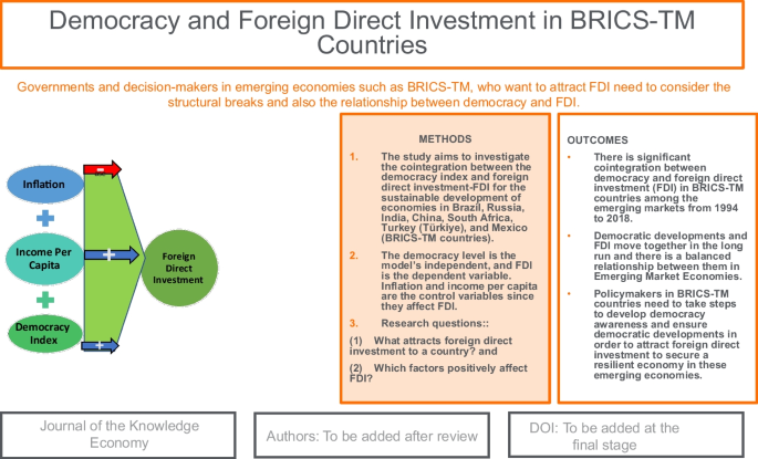
Economic Growth in Middle-Income Countries: The Role of Political Stability and Foreign Direct Investment

Short-Term Harm, Long-Term Prosperity? Democracy, Corruption and Foreign Direct Investments in Sino-African Economic Relations

Foreign direct investment and economic growth nexus in the presence of domestic institutions: a regional comparative analysis
Avoid common mistakes on your manuscript.
Introduction
Economies and governments require capital infusion to augment their production and employment levels. Underdeveloped and developing nations, despite having an abundance of land and labor, grapple with capital deficiencies. Consequently, these countries often seek foreign direct investment (FDI) to address this capital shortfall. Even emerging market economies are not immune to this phenomenon, with challenges intensifying globally post-COVID-19 pandemic. Khan et al. ( 2023 ) highlighted the pivotal role of institutional quality and good governance in attracting FDI. The need for FDI has grown exponentially in an increasingly globalized world characterized by interdependence among states. Democracy and the democratic status of states emerge as critical indicators of institutional quality. Kilci and Yilanci ( 2022 ) posit that the prolonged pandemic triggered the third most significant recession since the Great Depression of 1929 and the Global Financial Crisis of 2008–2009. Consequently, the demand for FDI has surged, positioning foreign investment as the foremost resource for fostering sustainable economic development. In light of the provided frame, this study addresses the following research questions:
What factors attract foreign direct investment to a country?
Which factors positively impact FDI?
Reviewing the existing literature reveals that scholars from diverse disciplines address similar questions using political variables like political stability and democracy levels or economic variables such as economic stability and natural resources . However, the impact of democracy on FDI is often overlooked . For example, studies by Baghestani et al. ( 2019 ) and Gür ( 2020 ) investigated variables like oil prices, exchange rates, exports, imports, and the global innovation index but seldom considered democracy’s role in attracting FDI . Similarly, studies examining the relationship between democracy and FDI, like those by Yusuf et al. ( 2020 ) and Ahmed et al. ( 2021 ), generally excluded data from BRICS-TM countries.
Li and Resnick ( 2003 ) assert that the two paramount features of modern international political economy are the proliferation of democracy and increased economic globalization . It has become apparent that FDI inflow is a manifestation of high-level globalization and the diffusion of democracy. According to the United Nations Conferences on Trade and Development (UNCTAD), 2002 data between 1990 and 2000, three-quarters of the total international foreign direct capital was directed toward democratic and developed countries (Busse, 2003 ).
The conceptualization of democracy, within both theoretical and historical frameworks, has been marked by inherent challenges (Suny, 2017 ). Aliefendioğlu ( 2005 ) defines democracy as the amalgamation of the ancient Greek terms “Demos” and “Kratos,” centered on the principle of self-governance by the people. In essence, democracy encompasses the utilization of popular sovereignty by and for the citizenry (Keser et al., 2023 ). Haydaroğlu and Gülşah ( 2016 ) contend that the contemporary manifestation of democracies is rooted in representative democracy, wherein individuals exercise their sovereignty by selecting representatives to act on their behalf. The spread of liberal or representative democracy is believed to be a driving force behind this shift in economic structures. The relational intersection between FDI flow and democratic mechanisms needs to be investigated. At this point, Voicu and Peral ( 2014 ) argue that economic development and modernization operate as background factors that affect the development of support for democracy. Therefore, an opinion emerges that there is an inevitable intersection between FDI flow and democratic mechanism.
Despite the sustained attention from academia and the public, the detailed understanding of democracy’s effect on FDI remains limited (Li & Resnick, 2003 ). There is a noticeable gap in the literature concerning studies investigating the impact of democracy on FDI, specifically in BRICS-TM countries , which are emerging markets that attract significant FDI. Moreover, the absence of structural break panel cointegration tests in previous analyses accentuates these gaps, forming the primary motivation for this research . The study aims to fill these voids by empirically examining the relationship between democracy and FDI using data from the emerging markets of BRICS-TM countries. These countries require substantial foreign capital and are crucial for the stable development of the global economy since they are expected to become pivotal centers in the multipolar world system. The study differs from other publications, employing unique methods, such as structural break panel cointegration tests, to address these objectives.
Reducing costs, increasing employment-oriented production, and enhancing export capacity are paramount in global competition. If a country cannot achieve these advancements with its existing potential and dynamics, attracting foreign capital becomes imperative, necessitating the creation of multiple attraction points to entice foreign direct investments. Consequently, attracting foreign capital is significant in today’s globalized world. This study provides insights into this pressing issue in the contemporary global competitive landscape by analyzing the long-term relationship between democracy and foreign direct investment. Considering their prominence in the world economy due to recent economic growth and competitive structures, the selection of BRICS-TM countries as a sample group underscores the study’s importance. The study acknowledges the strategic importance and increasing power of BRICS-TM countries, especially China and India, which have consistently attracted significant foreign capital in recent years. Using panel data analysis techniques that incorporate structural breaks addresses a crucial gap in the literature, offering a more accurate analysis of the democracy-foreign direct investment relationship in the BRICS-TM sample group. However, data constraints related to model variables alongside the limitations of evaluating results within the framework of the chosen sample group are acknowledged later in the “ Discussion ” section.
Lastly, there appears to be a gap in the existing literature concerning studies that investigate the impact of democracy on FDI flow in BRICS-TM countries . The countries that attract more FDI than others raise the question of whether their democracy level empirically influences the amount of FDI. Moreover, upon examining the limited studies exploring the relationship between democracy and FDI, it is evident that none applied the structural break panel cointegration test in their analyses. These gaps collectively serve as the primary motivation for this research. Thus, the study aims to address these gaps in the existing literature and scrutinizes whether there is cointegration between the level of democracy and FDI in a country by utilizing sample group data from emerging markets of BRICS-TM countries. This selection is significant as these countries are among emerging economies with considerable developmental potential. In essence, this study aims to empirically unveil the relationship between democracy and FDI , a crucial requirement for developing economies striving to attract more foreign capital for sustainable development . Additionally, this study employs distinctive methods, such as the structural break panel cointegration test, to investigate the subject, further elaborated in the “ Research Method and Econometric Analysis ” section.
In global competition, the imperative to reduce costs, increase employment-oriented production, and enhance export capacity is paramount. Given a country’s potential and dynamics, if these enhancements prove elusive, the necessity arises to attract foreign capital and establish various attraction points to incentivize foreign direct investments. Therefore, attracting foreign direct investment (FDI) to a country holds tremendous significance in today’s globalized world. Before investing, foreign capital rigorously assesses the potential profit opportunities and scrutinizes various socio-economic indicators, especially democracy. For these reasons, by analyzing the long-term relationship between democracy and foreign direct investment in the BRICS-TM sample, this study incorporates analyses and inferences regarding this crucial challenge in today’s globally competitive environment.
Furthermore, it is anticipated that the strategic importance and influence of BRICS-TM countries will continue to escalate in the upcoming years. Notably, countries in the sample group, particularly China and India, have consistently attracted substantial foreign capital, and their economies exhibit ongoing growth. As evident from the graphical analysis in the study, China stands out as the world leader in attracting foreign direct investment. Considering the economic size of Russia and Brazil, the geo-strategic location of Türkiye, and the natural resource wealth of China, India, and Mexico, it is apparent that these countries are central attractions for foreign direct capital. Events with significant consequences on the global stage, such as economic crises, wars, earthquakes, and elections, can induce substantial fluctuations and structural breaks in national economies. Hence, using panel data analysis techniques that allow for structural breaks in the study fills a critical gap in the literature. This approach provides a more accurate analysis of the democracy-foreign direct investment relationship in the BRICS-TM sample group. The primary limitation in the study’s analysis is the constraint arising from the variables included in the model. Additionally, selecting the BRICS-TM sample group as the focus on developing countries can be considered another limitation, restricting the evaluation of results within this specific sample framework. The study anticipates that the policy recommendations derived from the analysis findings will guide policymakers, market players, and new researchers.
The article is organized into the following sections: (1) “ Introduction ” section: This section initially furnishes broad information concerning the subject matter, elucidating the lacunae in the existing literature and delineating the limitations of the study. (2) “ Theoretical Frame and Literature Review ” section: Subsequently, the second section delves into the examination of the theoretical framework, scrutinizing the prevailing status of the literature. (3) “ Research Method and Econometric Analysis ” section: The third segment comprehensively addresses the research methodology employed and expounds upon the econometric analysis conducted. (4) “ Results ” section: The ensuing fourth chapter presents the study’s findings and results. (5) “ Discussion ” section: These results and findings are then systematically expounded upon in the fifth chapter within the context of the current literature. (6) “ Conclusion ” section: Culminating the study is a concluding section encapsulating the critical insights derived, followed by policy recommendations.
Theoretical Frame and Literature Review
As previously indicated, scarce studies have delved into the correlation between democracy and foreign direct investment (FDI). A comprehensive examination of the existing literature reveals a notable dearth of research focused on BRICS-TM countries, with most of them overlooking “democracy” as a variable and/or the connection between “democracy and FDI.” Conversely, researchers investigating FDI predominantly explore its associations with other variables, such as “exports and imports.”
The Status of the Literature on BRICS-TM Countries and Democracy and Foreign Direct Investment
The following two tables summarize the status of the current literature on the issue and its findings. In Table 1 , the literature on BRICS and/or BRIC + S + T + M countries, as well as its variables, methods, and findings, is given. Then, in Table 2 , the studies researching the relationship between democracy and FDI, their methodology, sample groups, and findings are summarized.
As can be seen in Table 1 , BRICS-TM countries were very rarely studied, and almost all of these studies neglected “democracy” as a variable and/or the relation between “democracy and FDI.” Alternatively, the studies that did examine FDI researched its relation with other variables such as export and import. Unique methods, such as structural break panel cointegration tests, were applied to investigate the issue, and this method comprises the novel part of the study. The details can be seen under the “ Research Method and Econometric Analysis ” section.
In summary, the literature review provided in Table 1 covers the relationship between democracy, foreign direct investment (FDI), and various other economic variables, focusing on BRICS-TM countries. Below is an analysis of the essential findings and gaps identified in the literature:
By applying AI (ChatGPT) to the information provided in Table 1 (studies on BRIC + S + T + M countries), key findings are double-checked and summarized below:
Limited focus on BRICS-TM countries: The literature review notes a scarcity of studies on BRICS-TM countries, with a lack of attention to the “democracy” variable in the context of FDI.
Variable relationships explored: Various studies investigate the relationships between different economic variables and FDI, such as oil prices, exchange rates, gross domestic product (GDP), international tourism, economic output, carbon emissions, exports, imports, and innovation.
Diverse methodologies: Researchers employ diverse methodologies, including directional analysis, panel ARDL cointegration, survey research, and panel cointegration, to analyze the relationships among variables.
Within this frame, a summary of the studies investigating the relationship between democracy and FDI or using similar variables is given in Table 2 .
As presented in Table 2 , none of the above studies analyzed the relationship among democracy, FDI, inflation , and GDP variables for BRICS-TM countries. In addition, none of the studies applied a structural break panel cointegration test in their analysis. All these gaps motivate the authors of this study to conduct such research.
Additionally, applying AI (ChatGPT) to the information provided in Table 2 , key findings from Table 2 are double-checked and summarized below (studies on the relationship between democracy and economics):
Limited studies on democracy and FDI in BRICS-TM: The literature highlights a gap in research, as none of the studies in Table 2 specifically analyze the relationship between democracy, FDI, inflation, and GDP variables in BRICS-TM countries.
Contradictory findings on democracy and economic growth: The studies in Table 2 present contradictory findings on the impact of democracy on economic growth. Some find a positive and significant effect, while others do not establish a significant relationship.
Methodological variety: Various methods, such as dynamic fixed effects, panel data regression analysis, panel cointegration, and causality analysis, are employed to explore the relationships between democracy, FDI, and economic growth.
Upon inspection of the limited studies, contradictory results emerge, even when employing data from diverse sample groups. An illustrative example is found in the work of Busse ( 2003 ), whose research can be summarized as follows:
Results from regression analysis between FDI and democracy reveal that analogous to studies by Rodrik ( 1996 ) and Harms and Ursprung ( 2002 ), multinational corporations (MNCs) exhibit a preference for countries where political rights and freedoms are legally and practically safeguarded.
Countries that enhance their democratic rights and freedoms tend to attract more FDI per capita than predicted (Busse, 2003 ).
Li and Resnick ( 2003 ) posited that investors typically favor regimes with advanced democracy and robust legal systems over states where their properties are at risk in dictatorial regimes. From this standpoint, one can infer that a significantly high level of democracy correlates with a markedly high level of FDI. In other words, property rights violations are diminished in developing countries with robust democracies, leading to increased FDI levels (Li & Resnick, 2003 ).
However, Haggard ( 1990 ) presents a contrary perspective, arguing that authoritarian regimes may appeal more to investors seeking to safeguard their economic assets and properties. An amalgamation of opposing views arises: investors from countries with underdeveloped democracies prefer collaboration with authoritarian regimes, whereas investors from developed nations lean toward familiar democratic regimes.
Despite the contradictory and complex findings from the limited number of studies on the potential relationship between democracy and FDI, it is contended that two influential factors contribute to investment flow toward countries with legally guaranteed and well-developed democratic rights. Firstly , as proposed by Spar ( 1999 ), a transition occurs from critical sectors like agriculture and raw materials to production and tertiary sectors in the flow and stock structure of FDI in developing countries. Secondly , there is a transformation in the interest and motivation of multinational enterprises toward developing countries based on sectoral development (Busse, 2003 ). This underscores the impact of democratic organizations established to secure democratic rights on FDI. In instances where poor democratic governance renders a country less appealing to foreign investors, the country faces a dilemma: choosing between the limited options of “loss of foreign capital” or “democratization” (Li & Resnick, 2003 ). Spar ( 1999 ) emphasizes that as the reliance on governments and their policies decreases, the need for a more democratic environment, a reliable and stable legal system, and appropriate market conditions becomes increasingly crucial for the overall well-being of the country’s economy.
Upon scrutinizing the most recent studies on the subject, a trend of contradictory findings becomes apparent. For instance, Yusuf et al. ( 2020 ) found that the democracy coefficient, as a variable signifying its impact on economic growth, lacks significance for West African countries in the short and long run. In contrast, Putra and Putri ( 2021 ) asserted that “democracy has a positive and significant effect on economic growth in 7 Asia Pacific countries.” Similar to Yusuf et al., in a panel data analysis encompassing the period from 1970 to 2014 and involving 115 developing countries, Lacroix et al. ( 2021 ) concluded that “democratic transitions do not affect foreign direct investment (FDI) inflows.”
A comprehensive review of existing empirical studies reveals a notable scarcity in the number of inquiries into the relationship between democracy and foreign direct investment (FDI) (Li & Resnick, 2003 ). Moreover, the available studies yield contradictory results on this matter. Addressing this issue, it is noteworthy that Oneal ( 1994 ) conducted one of the initial qualitative examinations on the impact of regime characteristics on FDI. Despite not identifying a statistically valid relationship between regime type and FDI flow, Oneal’s research is an early exploration of this intricate relationship.
Explorations into the connection between investor behavior and political regime characteristics, particularly in determining whether democratic or authoritarian features foster more foreign direct investment (FDI), have yielded divergent outcomes. Derbali et al. ( 2015 ) found a statistically significant relationship between FDI and democratic transformation. Through an econometric analysis encompassing a sample of 173 countries, with 44 undergoing democratic transformation between 1980 and 2010, the authors observed a substantial increase in FDI flow associated with democratic transitions.
Castro ( 2014 ) conducted a test examining the relationship between foreign direct investment (FDI) flow (the ratio of FDI flow to GDP) and indicators of “democracy” and “dictatorship” using a dynamic panel data model. Despite the analysis results failing to furnish evidence supporting a direct connection between FDI and democracy, the author emphasizes that this outcome does not negate the impact of political institutions on the flow of FDI. According to Mathur and Singh ( 2013 ), their study stands out as the inaugural examination focusing on the “importance given to economic freedom rather than political freedom” in the decision-making process of foreign investors. The authors concluded that contrary to conventional expectations, even democratic countries may attract less foreign direct investment (FDI) if they do not ensure guaranteed economic freedom. Malikane and Chitambara ( 2017 ) conducted a study exploring the relationship between democracy and foreign direct investment (FDI), employing data from eight South African countries from 1980–2014. The research findings indicate a direct and positive impact of FDI on economic growth due to the robust democratic institutions emerging as crucial catalysts in the respective sample countries.
Consequently, Malikane and Chitambara’s ( 2017 :92) study suggests that the influence of FDI on economic growth is contingent upon the level of democracy in the host country. Upon scrutinizing the studies above, a pattern of conflicting findings emerges concerning the relationship between the level of democracy and the influx of foreign direct investment (FDI) to a country . Studies commonly emphasize that the impact of democracy on FDI depends upon each country’s developmental stage. The prevalence of confusion, varying findings, and conflicting results underscores the significance of empirical analyses on this matter. A comprehensive examination of the overview identified gaps, and the need for new research is detailed under the subsequent subheading.
Overview of the Literature, Identified Gaps, and Requirements for New Research
After a detailed overview of the existing literature, the main features and gaps can be identified as follows:
Limited studies on democracy and FDI: The literature notes a scarcity of studies examining the relationship between democracy and FDI, and existing studies present conflicting results.
Context-dependent impact of democracy: Contradictory findings suggest that democracy’s impact on FDI may vary depending on a country’s development level.
Gap in BRICS-TM studies: The identified gap in the literature is the lack of research specifically addressing the relationship between democracy and FDI in BRICS-TM countries. The need for a structural break panel cointegration test is also emphasized.
Influence of political institutions: Some studies argue that solid democratic institutions positively influence FDI, while others suggest that economic freedom, rather than political freedom, may be more crucial for attracting FDI.
Requirements for new research: To fill the gap in the literature, new research should be conducted specifically targeting BRICS-TM countries.
Thus, when c onsidering the contradictory findings, future studies should explore the contextual factors influencing the relationship between democracy and FDI in different country settings. Conducting longitudinal analyses could provide insights into the dynamic relationship between democracy and FDI over time. Comparative studies between countries with different levels of democratic development can help in understanding the nuanced impact of democracy on FDI. Last but not least, given the emphasis on structural break panel cointegration tests, future research could incorporate these analytical tools for a more comprehensive understanding of the relationships under consideration.
Last but not least, Olorogun ( 2023 ) conducted research using data from sub-Saharan countries from 1978 to 2019 and found a “long-run covariance between sustainable economic development and foreign direct investment (FDI)” and a “significant level of causality between economic growth and financial development in the private sector, FDI, and export.” So, if a significant relationship can be found between democracy and foreign direct investment, the results may also provide a useful assessment for sustainable development.
In summary, while the literature review reveals valuable insights into the complex relationship between democracy, FDI, and economic variables, there is a clear need for more targeted research in the context of BRICS-TM countries by further exploration of the contextual factors influencing these relationships.
Research Method and Econometric Analysis
This section of the study delves into the analysis methods and interpretations of the relationship between democracy and foreign direct investment (FDI). The presentation encompasses the dataset and model specifications concerning the variables under scrutiny. Specifically, analyses were conducted utilizing econometric analysis programs, namely, EViews 12 , Gauss 23 , and StataMP 64 . The study culminated with interpreting findings and formulating policy recommendations based on the results obtained.
Data Set and Model
The study scrutinized the hypothesis to address the initial research inquiry, asserting a correlation between democracy and foreign direct investment (FDI). The research targeted BRICS-TM countries (Brazil, Russia, India, China, South Africa, Türkiye, Mexico) recognized for their increasing prominence in the global economy and anticipated growth in strategic significance. These seven emerging markets were chosen due to their demonstrated potential to attract FDI. The research covered annual data spanning 1994–2018 by employing panel data analysis techniques capable of accommodating structural breaks. Both democracy and foreign direct investments are susceptible to the influence of local and global dynamics, which can induce significant disruptions in the variables.
Consequently, the study utilized tests allowing for structural breaks to enhance the robustness of the analyses. The investigation aimed to uncover the long-term relationship between foreign direct investment and democracy , a critical indicator of economic development for emerging markets in recent years. The model developed for examining the relationship between democracy and foreign direct investment within the specified sample and data range is represented by Eq. 1 :
In the model, cross-section data is represented by i = 1, 2, 3,…. N , while the time dimension is represented by t = 1, 2, 3,….. T , and the error term is by ɛ.
The study’s model setup and variables were adapted from Yusuf et al. ( 2020 ), Putra and Putri ( 2021 ), and Lacroix et al. ( 2021 ) in the literature. Figure 1 shows the research design.

Research design
Table 3 shows the variables and data sources used in the model.
The study designated foreign direct investment (FDI), denoted as LNFDI, as the dependent variable. The independent variable was conceptualized as the democracy variable (DEMOC). To account for potential influencing factors, inflation (INF) and per capita income (PGDP) variables, known to impact FDI, were introduced into the model as control variables to draw upon insights from the existing literature. In the context of panel data analyses, selecting control variables involves consulting the literature to identify factors with substantial influence on the dependent variable. When examining factors impacting foreign direct investment (FDI), a frequently encountered category comprises various macroeconomic variables, among which inflation and per capita income are recurrently employed. Given the study’s sample composition—comprising the BRICS-TM countries—these two variables were incorporated into the model as control variables. This decision was motivated by their recurrent utilization in the literature and their direct relevance to foreign direct investments and production costs. Furthermore, the inclusion of these variables addressed a shared data constraint.
During the data collection phase, the study utilized indices reflecting “political rights” and “civil liberties,” which were acknowledged indicators of “democracy” in the literature. These indices, sourced from the Freedom House Database ( 2020 ), were incorporated into the analysis by calculating their means, which were then used as values for the democracy variable. This approach aligns with the practices of several researchers in the existing literature, such as Kebede and Takyi ( 2017 ), Doucoligaos and Ulubasoglu ( 2008 ), and Tavares and Wacziarg ( 2001 ), who have employed this index. The index operates on a scale from 1 to 7, where 1 represents the highest state of democracy and 7 corresponds to the lowest state. To facilitate analyses, calculations, and interpretation, the index values were scaled to ensure a range between 0 and 100.
Freedom House assesses the degree of democratic governance in 29 countries from Central Europe to Central Asia through its annual “Nations in Transit” report. The democracy score encompasses distinct ratings on various facets, including national and local governance, electoral processes, independent media, civil society, judicial framework and independence, and corruption. Most researchers (Dolunay et al., 2017 ; Martin et al., 2016 ; Osiewicz & Skrzypek, 2020 ; Steiner, 2016 ) frequently utilize the data provided by Freedom House in their studies. In addition to the independent variable of democracy (DEMOC), the model integrates control variables influencing FDI. Capitation (LNPGDP) and inflation (INF) variables were incorporated within this framework. A review of the existing literature reveals that factors affecting FDI, including inflation and per capita income, have been employed in models by researchers (Botric & Skuflic, 2005 ; Chakrabarti, 2001 ; Jadhav, 2012 ; Ranjan & Agraval, 2011 ; Vijayakumar et al., 2010 ).
In the literature, various variables such as “trade openness, level of human capital, unemployment rates, government supports, tax costs,” which are believed to influence foreign capital, are employed as control variables in models. On the other hand, in some research, the impact of institutional quality, such as democracy and governance, on environmental quality is studied. Within this frame, Shahbaz et al. ( 2023 ) found that “institutional quality variables impacted environmental quality differently. In this sense, it is detrimental for policymakers to consider concerted measures to decrease institutional vulnerabilities and reduce the level of the informal economy.” However, in this study, inflation and per capita income variables were chosen due to their prominence as the most frequently used variables in the literature (detailed in the “ Theoretical Frame and Literature Review ” section) and their comprehensive impact on foreign direct capital in terms of macroeconomics.
Furthermore, a shared data problem is evident in all variables from 1994 to 2018 for the BRICS-TM country sample group, particularly in variables other than the control variables in the model. Nevertheless, these issues have yet to be encountered as inflation and per capita income variables are comprehensive and fall within general macroeconomic data. Additionally, including many control variables in the model might obscure the significance of the effect on the dependent variable in hypothesis tests examining the relationship between democracy and foreign direct investment. Consequently, real GDP data, rather than nominal, were utilized in the analysis, and the logarithm of the data was represented as LNGDP.
As explored earlier, foreign investors prioritize economic freedom over political freedom when making investment decisions (Mathur & Singh, 2013 ). In this context, the assurance of economic liberty and the legal protection of property rights may be linked to the level of democracy, particularly in developed countries. This condition explains why the relevant variables should be incorporated into the model and tested. The logarithm of FDI (LNFDI) and per capita income (LNPGDP) variables were employed in the analyses. The rationale behind the logarithmic transformation lies in its capacity to facilitate the interpretation of analysis results and standardize variables on a specific scale. Additionally, taking logarithms of series does not result in information loss in data; it also aids in mitigating autocorrelation issues and allows the series to exhibit a normal distribution.
Econometric Method
The primary motivation behind the conducted study is to investigate the impact of the variable “democracy” on foreign direct investments through newly developed panel data analysis tests that allow for structural breaks, which are not commonly used in political science. In this regard, the study aims to be one of the pioneering works testing the relationship between variables related to political science and economics with an interdisciplinary perspective through innovative empirical studies. The methodological framework of this study, which analyzes the relationship between democracy and FDI through annual data from the 1994–2018 periods using panel data analysis and causality test, is outlined below:
Graphical representation of variables and analysis of descriptive statistics,
CD lm1 (Breusch & Pagan, 1980 ), CD lm1 , and LM adj tests (Pesaran et al., 2008 ) were used in the analysis to find the presence of cross-section dependence of variables.
Panel LM test (Im, Lee, & Tieslau, 2010 ) determined whether variables in the model have a unit root.
Delta test (Pesaran & Yamagata, 2008 ) was used to determine the homogeneity or heterogeneity of variables.
Cointegration test with multiple structural breaks (Westerlund & Edgerton, 2008 ) was conducted to determine the presence of cointegration between variables.
Kónya’s causality test (Kónya, 2006 ) was conducted to investigate the existence of causal relationships between variables.
In terms of methodology, the study aims to address a significant gap in the literature on democracy. Given the chosen sample group and the specified period, it becomes evident that structural changes must be considered in the analysis because the variables of democracy and foreign direct investment are particularly susceptible to global developments, leading to substantial shifts in the markets. A literature review indicates a preference for general country-based time series analyses over new-generation tests, with classical panel data analyses commonly employed for the selected country group. In summary, an examination of the literature reveals that studies on this issue predominantly rely on first- and second-generation linear panel data analysis techniques. Therefore, incorporating unit root and cointegration tests is crucial in significantly contributing to the literature, particularly by acknowledging and addressing structural breaks in the study. Additionally, it aligns with the theoretical framework that variables such as democracy and foreign direct capital investments, susceptible to the influence of global developments, are prone to structural changes. Consequently, employing panel data analysis techniques with structural breaks gains significance and enhances the motivation and scientific robustness of the study, mainly when a substantial data range is available.
The study focuses on the BRICS-TM countries: Brazil, Russia, India, China, South Africa, Türkiye Footnote 1 (Turkey), and Mexico . These nations have gained prominence in the global economy, and their strategic significance is anticipated to grow. The selection of this sample group is based on their demonstrated high performance and potential to attract substantial foreign direct investment globally. The study’s unique contribution lies in its examination of the impact of the democracy variable on foreign direct investments within this specific country group, employing innovative techniques not commonly found in the existing literature. Furthermore, the potential increase in foreign direct investment within these countries is expected to influence national and per capita incomes positively. The continuous enhancement of economic well-being and the rising accumulation of foreign direct investments could position these countries as new focal points of attraction in the medium and long term, fortifying their appealing characteristics.
Descriptive Statistics and Graphical Analysis of Variables
Graphical analyses provide valuable insights into the changes and fluctuations of variables over the years in econometric studies. The visual representation and interpretations of the study variables are presented in Fig. 2 .

Graphical representation of variables
The graphical analysis reveals the trend and volatility of FDI over the study period (1994–2018). Peaks and troughs may indicate significant events or economic shifts influencing FDI.
Democracy index: The graphical representation illustrates the changes in the democracy index across the selected countries. Distinct patterns or shifts may be observed, indicating periods of democratic development or regression.
Inflation (INF): The inflation variable is depicted graphically, highlighting its trajectory over the analyzed years. Fluctuations in inflation rates may correlate with economic events impacting FDI.
Per capita income (PGDP): The per capita income variable is visually presented, demonstrating its variations and trends. Per capita income changes can influence countries’ attractiveness for foreign investments.
These graphical analyses serve as a foundation for understanding the dynamics of the variables under investigation and provide a visual context for further econometric interpretations.
So Fig. 2 provides a comprehensive overview of the variables examined in the study. The following key observations can be made:
Foreign direct investment (FDI): China stands out as the leader in attracting the highest FDI among the BRICS-TM countries. South Africa exhibits the lowest FDI levels in the sample group.
Democracy index: China also holds the highest score in the democracy index, indicating its position as the most democratic among the selected countries. South Africa, on the other hand, has the lowest democracy index score.
Per capita income (PGDP): Russia demonstrates the highest per capita income among the countries, suggesting a relatively higher economic well-being. India, conversely, has the lowest per capita income in the sample group.
Inflation (INF): Russia and Türkiye experience the highest inflation rates, while other countries exhibit fluctuating patterns at lower and similar levels.
Table 4 provides a detailed overview of the descriptive statistics for the variables under consideration. The following key statistics offer insights into the central tendencies and variations within the sample group.
The analysis of the basic descriptive statistics in Table 4 yields several noteworthy findings:
Kurtosis values: The INF variable stands out with a kurtosis value exceeding 3, indicating a sharp peak and heavy tails in its distribution. All other variables exhibit kurtosis values below 3, suggesting relatively normal distributions without excessively heavy tails.
Skewness values: LNFDI and LNPGDP variables display negative skewness values, suggesting a longer left tail in their distributions. DEMOC and INF variables exhibit positive skewness values, indicating longer right tails in their distributions.
Jarque–Bera test: The Jarque–Bera test results indicate that the variables are statistically significant and deviate from a normal distribution. This departure from normality suggests that certain factors or events influence the distributions of the variables.
These findings provide insights into the shapes and characteristics of the variable distributions. As indicated by skewness and kurtosis values, the deviations from normality suggest that the variables may be subject to specific influences or events, contributing to their non-normal distributions. Researchers should consider these distributional characteristics when interpreting the results and drawing conclusions from the dataset.
Cross-section Dependence Test
The escalating interdependence among countries in global economies has rendered them susceptible to the impact of positive or negative developments in one nation affecting others. This phenomenon directly results from the deepening global integration associated with globalization. Consequently, econometric studies must incorporate cross-section dependence tests to gauge the extent of interaction between nations. Such tests aim to quantify how a shock in one country reverberates across borders, influencing other countries of the global economic landscape.
Studies addressing cross-section dependency (Andrews, 2005 ; Pesaran, 2006 ; Phillips & Sul, 2003 ) emphasize that failing to account for cross-section analysis may lead to biased and inconsistent results. Thus, all analyses should consider cross-sectional dependence in relevant studies (Breusch & Pagan, 1980 ; Pesaran, 2004 ).
The tests used to determine cross-section dependence were as follows:
When the time dimension is greater than the cross-section dimension ( T > N ), analyses were conducted using Breusch and Pagan’s ( 1980 ) CD lm1 test.
In cases when the time dimension is equal to the cross-section dimension ( T = N ), the CD lm2 test (Pesaran, 2004 ) was used to conduct analyses.
In cases when the time dimension was smaller than the cross-section dimension ( T < N ), analyses were conducted by CD lm test (Pesaran, 2004 ).
In cases when the time dimension is both smaller and greater than the cross-section dimension, analyses were conducted (LM adj ) test (Pesaran et al., 2008 ).
This study’s analysis focuses on the relationship between democracy and FDI across BRICS-TM countries, involving seven countries. With annual data spanning 1994–2018, the cross-section dimension is denoted by N = 7 and the time dimension by T = 25. Given that T > N , the study utilized the CD lm1 test (Breusch & Pagan, 1980 ) and CD lm1 and LM adj tests (Pesaran et al., 2008 ).
Given that T > N for the countries and time dimension, the decision-making is informed by the results of the CD lm1 and LM adj tests. Notably, LM adj test results were prioritized, considering the potential bias in cross-section dependency tests associated with the CD lm1 test. The findings of the cross-section dependence tests are presented in Table 5 .
Upon reviewing Table 5 , it is evident that the probability values for all variables are less than 0.01. Consequently, based on the LM adj test results, the null hypothesis stating “there is no dependence between sections” is rejected, while the alternative hypothesis suggesting “cross-section dependence between sections” is accepted.
The outcomes of the tests align with the characteristics of the contemporary global landscape, where any impactful event or development in one of the BRICS-TM countries has reverberations across others. Whether positive or negative, changes in one BRICS-TM nation can influence others, particularly in areas related to foreign direct investment (FDI) and democracy. As a result, policymakers in these countries should craft their future strategies with a keen awareness of this interconnectedness and the potential spillover effects on FDI and democracy. Indeed, the obtained result is consistent with theoretical expectations. The observed interdependence and influential power of the BRICS-TM country group align with the current dynamics of the globalized world. Their growing significance in the world economy and their strategic importance reinforces the decision that developments within these countries have substantial implications beyond their borders. This outcome urges the need for a nuanced approach to respond to the interconnected nature of these nations in the contemporary global landscape.
Panel Unit Root Test
In the initial phase of the econometric analysis, the stationarity of the variables in the models was determined through unit root analyses to address the spurious regression problem. Accurate results cannot be obtained when a unit root is present in a series of variables (Granger & Newbold, 1974 ). In panel data analysis, the primary consideration in stationarity tests is whether the countries are independent of each other or not. Unit root tests in panel data analysis comprise first- and second-generation tests, each with distinct characteristics. The first generation of unit root tests is further divided based on the homogeneity and heterogeneity assumptions of the countries. Some authors conducted tests under the homogeneity assumption (Breitung, 2005 ; Hadri, 2000 ; Levin et al., 2002 ), while some others pursued their analysis under the heterogeneity assumption (Choi, 2001 ; Im et al., 2003 ; Maddala & Wu, 1999 ).
Additionally, second-generation tests incorporate cross-section dependency into their analyses, whereas first-generation tests do not account for it. Given the dynamics of the global world, the use of second-generation tests in the literature is deemed more beneficial, as it is more realistic to assume that other countries will be affected by a shock experienced by one of the countries in the panel. Panel unit root tests have gained broader acceptance in time series analysis due to their ability to provide more meaningful results than standard stationarity tests. In recent years, there has been a preference for tests that allow for structural breaks, especially in series sensitive to economic variations such as foreign trade, exchange rates, and foreign capital. Hence, this study utilized panel unit root tests that consider structural breaks to assess the stationarity of variables susceptible to cyclical fluctuations, including democracy, inflation, per capita income, and FDI. Conducting stationarity tests without accounting for structural breaks can yield misleading results, making panel LM unit root tests with structural breaks the method of choice for this study.
The panel LM test (Im, Lee, & Tieslau, 2010 ) examines series in models with a level and trend, considering single and two breaks. In this study, analyses with a single break were preferred due to the shortness of the specified time interval and the events expected to cause breaks in the given period. The LM test statistics were employed to assess the hypothesis of “there is a unit root” (ϕ i = 0). Compared to others, a distinctive feature of this test is its allowance for different breaking times for different countries. Moreover, it permits a structural break under both zero and alternative hypotheses, providing an additional advantage. The asymptotic distribution of the test follows the standard normal distribution, and it remains unaffected by the presence of a structural break. Table 6 presents the stationarity analysis results of the series for seven countries based on the model allowing breaks in level.
The analysis of Table 6 yields the following observations:
In unit root models allowing for a constant break, it is evident that all variables in the panel become stationary when their differences are calculated. In other words, since the series are stationary for the entire panel at the I(1) level, the necessary conditions for cointegration tests are met. The cointegration test indicates that global and local developments in countries cause structural breaks when considering these break dates.
On a country basis, the following conclusions can be drawn from Table 6 :
For the series whose differences are calculated, the FDI variable is stationary at the level value in Russia and India, while the same variable is stationary in India and Türkiye.
The per capita income variable is stationary at a level value only in Türkiye. However, the same variable is stationary in Brazil, India, and Türkiye for the series whose differences are computed.
The inflation variable is stationary at the level value in South Africa and Mexico. However, the same variable is stationary for the series whose differences are computed in Brazil, Russia, and China.
The democracy variable is stationary at the level value in Brazil, South Africa, and Türkiye. However, the variable is stationary in Brazil, Türkiye, and Mexico for the series whose differences are computed.
Table 7 shows the stationarity analysis results of seven countries based on the model that allows breaks in level and trend.
The results in Table 7 can be analyzed based on the following points:
General panel evaluation: Foreign direct investment (FDI) and per capita income variables are stationary at the level values when the panel is considered whole. Taking the difference of these variables increases the degree of stationarity. Inflation and democracy variables, among the other variables in the model, are stationary in the series when the difference is taken. However, they exhibit unit root characteristics at the level values. Overall, all series are stationary at the I(1) level with structural breaks for the entire panel. This suggests that the necessary conditions for the cointegration test are met. The dates of structural breaks indicate that social, political, and economic developments may have caused these breaks in the BRICS-TM countries included in the sample . These findings imply that significant events and changes in the socio-political and economic landscape of the BRICS-TM countries likely influence the structural breaks in the series.
Results from Table 7 can be interpreted on a country-specific basis as follows:
Brazil: FDI and per capita income are stationary at the level value. Inflation is stationary at the level, while democracy is stationary at the difference.
Russia: FDI and per capita income are stationary at the level value. Inflation is stationary at the level, while democracy is stationary at the difference.
India: FDI is stationary at the level value. Per capita income is stationary at the level, while inflation and democracy are stationary at the difference.
China: FDI is stationary at the difference. Per capita income is stationary at the level, while inflation and democracy are stationary at the difference.
South Africa: FDI is stationary at the level value. Per capita income is stationary at the level, while inflation and democracy are stationary at the difference.
Türkiye: FDI is stationary at the level value, per capita income is stationary at the level, and inflation and democracy are stationary at the difference.
Mexico: FDI is stationary at the difference. Per capita income is stationary at the level, while inflation and democracy are stationary at the difference.
These country-specific findings indicate variations in the stationarity characteristics of the variables, highlighting the importance of considering individual country dynamics in the analysis. The results of the panel unit root tests, both with and without structural breaks, provide insights into the stationarity of the variables. The interpretation suggests that a shock to one of the countries included in the model can lead to permanent effects that do not dissipate immediately. As confirmed by the tests, the non-stationarity of the series establishes the necessary condition for cointegration tests.
Moreover, when the same tests are conducted by taking the first-order differences of all series to achieve stationarity, it is observed that the variables become stationary at the I(1) level. This indicates that the variables are integrated in the first order, aligning with theoretical expectations. The I(1) characteristic implies that the variables exhibit a tendency to return to equilibrium after a shock, supporting the notion of long-run relationships among the variables.
Homogeneity Test of Cointegration Coefficients
The homogeneity of coefficients plays a crucial role in determining the relationship between variables in panel data studies. It helps organize subsequent tests used in the analysis. The homogeneity test examines whether the change in one country is affected at the same level by other countries. Coefficients are expected to be homogeneous in models for countries with similar economic structures, while they may be heterogeneous for countries with different economic structures. Pesaran and Yamagata ( 2008 ) developed the delta test based on Swamy ( 1970 ) to determine whether the slope parameters of cross-sections are homogeneous. The null hypothesis for this test is “slope coefficients are homogeneous.” Homogeneity, in the context of panel data analysis, implies that the coefficients of the slopes are the same for all units or entities within the panel. On the other hand, heterogeneity indicates that, at least in one of the entities, the slope coefficients differ from those in the rest of the panel. Testing for homogeneity helps assess whether the relationship between variables is consistent across all units or if there are significant variations.
As seen in Table 8 , the delta homogeneity test was performed to determine whether the slope coefficients of the model differ between units.
The delta test results indicate that the slope coefficients vary between units in the long term, given that the probability values for both test statistics are smaller than 0.05, as presented in Table 8 . This result suggests that the variables exhibit heterogeneity, implying that the relationships between variables are inconsistent across all units over the long term. The obtained result aligns with expectations and is consistent with the theory, indicating that the countries within the BRICS-TM sample exhibit different structures, and the coefficients are heterogeneous. This result suggests that the relationship between variables varies across these countries, emphasizing the sample group’s diverse economic characteristics and behaviors.
Panel Cointegration Test with Structural Break
Different methods are employed to determine the existence of long-term cointegration among the model’s variables. One set of methods is first-generation tests, which do not require cross-section dependence. The second set includes second-generation tests that consider cross-section dependence but do not incorporate structural breaks (Koç & Sarica, 2016 ). To obtain realistic and unbiased results, it is crucial to conduct tests that take structural breaks into account in cointegration analyses. Therefore, the panel cointegration test-PCWE (Westerlund & Edgerton, 2008 ) was employed, given that the series is stationary at the I(1) level.
PCWE was developed based on unit root tests that utilize Lagrange multiplier (LM) statistics, obtained from multiple repetitions (bootstrap). The merits of this test can be succinctly summarized as follows (Koç & Sarica, 2016 ; Göçer, 2013 ):
It takes into account cross-section dependency and structural breaks.
It accommodates heteroscedasticity and autocorrelation.
It identifies breaks at different dates for each country in terms of both constants and slopes.
Potential inherent problems in the model can be addressed with fully adjusted least squares estimators.
This test is effective in yielding reliable results even with small sample sizes.
This study opted for PCWE tests, given their robust characteristics. Additionally, considering the limited number of countries in the sample and the anticipation of few structural breaks in the specified period, the PCWE test was the preferred choice. As depicted in Table 9 , the determination of statistically significant cointegration between variables is made based on the significance levels of the probability values.
As indicated in Table 9 , cointegration is observed at a 5% significance level in the regime change model and a 1% significance level in the model without a break. The presence of cointegration suggests a long-term relationship between the variables of democracy and FDI in BRICS-TM. In simpler terms, democratic developments and FDI are correlated over the long run, indicating a balanced relationship between them. Future researchers may explore the direction of these variables across different samples. This study specifically tested the existence of a long-term relationship between FDI and democracy, and the inclusion of structural breaks was found to be significant. Governments and decision-makers, particularly in developing countries like BRICS-TM, should consider the relationship between democracy and FDI by taking structural breaks into account to attract foreign investment effectively. Therefore, it is emphasized that “any development related to democracy has the potential to influence FDI, and considering this factor is beneficial in the formulation and implementation of socio-economic policies.” No cointegration is observed in the “change at level” model. Indeed, the obtained results align with the study’s hypothesis. Considering the periods of structural breaks in the countries within the sample, it becomes evident that a long-term relationship exists between the variables incorporated into the model. This issue underscores the importance of considering not only the overall relationship between democracy and FDI but also the specific historical contexts and transitions in individual countries that might contribute to this relationship.
Regarding structural breaks in countries in the sample within the scope of cointegration in the regime change model, local and global developments, in general, cause breaks. The reasons for structural break dates in the sample countries are given in Table 10 .
The following items can be aligned with the breaking dates provided in Table 10 :
A recovery in macroeconomics and positive expectations toward agreements with the IMF became prominent after Russia’s transition economies in 1996.
2000 in Brazil is known as the period when the rapid growth trend started after passing the targeted inflation after the 1999 Russian Crisis.
Membership of China in the International Trade Union was evaluated as an essential development in the global economy in 2001.
Experiencing the biggest crisis in history in Türkiye in 2002 and starting a dominant single-party regime were remarkable developments.
The 2005 Election results in Mexico and the hurricane disasters, including an 8.7-magnitude earthquake, created significant socio-economic problems that year.
The ANC party’s coming to power alone in South Africa in 2009 was commented on as a consistent process for the national and regional economy; this situation also removed a series of uncertainties.
The devaluation experienced in India in 2016 has created a significant break.
Of course, the impact of such structural breaks should be considered. Toguç et al. ( 2023 ) argued that “differentiating these short-term and long-term effects has implications for risk management and policymaking.” Since structural break increases risks and uncertainty, foreign capital prefers to invest in other destinations.
Kónya’s Causality Test
This test (Kónya, 2006 ) investigates the existence of causality between variables using the seemingly unrelated regression (SUR) estimator (Zellner, 1962 ). One advantage of this test is that the causality test can be applied separately to the countries that make up the heterogeneous panel. Another important advantage is that it is unnecessary to apply unit root and cointegration tests, as country-specific critical values are produced. According to the test results, if the Wald statistics calculated for each country are greater than the critical values at the chosen significance level, the null hypothesis of “no causality between the variables” is rejected. In other words, a Wald statistic greater than the critical value indicates that there is causality between the variables.
The Kónya causality test results provided in Table 11 revealed a causality from democracy (DEMOC) to FDI at a 1% significance level in Mexico, 5% in China, and 10% in Russia. In addition, from FDI to democracy (DEMOC), there is causality at a 5% significance level in Mexico and a 10% significance level in Russia.
According to the results in Table 12 for the causality between foreign direct investment (FDI) and PGDP, the Kónya causality tests revealed a one-way causality from PGDP to FDI at a 10% significance level in Mexico.
According to the results provided in Table 13 for the causality between foreign direct investment (FDI) and inflation (INF), the results of the Kónya causality tests revealed a one-way causality from inflation to FDI at a 10% significance level in Türkiye and, conversely, a one-way causality from FDI to inflation at a 10% significance level in South Africa.
The study investigated the nexus between democracy and foreign direct investment (FDI) using annual data from a sample of seven countries within emerging markets from 1994–2019. According to cross-section dependence test results, all variables’ probability values were less than 0.01, indicating significant cross-section dependence. The rejection of the null hypothesis, stating “there is no dependence between sections” in favor of the alternative hypothesis suggesting “there is cross-section dependence between sections,” aligns with the contemporary global landscape. In today’s interconnected world, any impactful event or development in one of the BRICS-TM countries has reverberations across others, particularly in areas related to FDI and democracy. These findings underscore the imperative for governments and policymakers in these countries to craft future strategies with a keen awareness of this interconnectedness and the potential spillover effects on FDI and democracy.
Furthermore, the outcomes of the panel unit root test indicate that all variables in the panel become stationary at the I(1) level when their differences are calculated, meeting the necessary conditions for cointegration tests. This result suggests that global and local developments in countries cause structural breaks when considering these break dates. Variations in stationarity characteristics of variables were observed on a country basis, highlighting the importance of considering individual country dynamics in the analysis.
The delta homogeneity test results suggest that the variables exhibit heterogeneity, implying that the relationships between variables are inconsistent across all units over the long term. This aligns with expectations and emphasizes the diverse economic characteristics and behaviors within the sample group of BRICS-TM countries.
The Westerlund-Edgerton cointegration test results reveal significant cointegration between variables, observed at a 1% significance level in the model without a break and a 5% level in the regime change model. This result signifies a sustained relationship between FDI and democracy in BRICS-TM countries over the long term. Future researchers may explore the direction of these variables across different samples, while governments and decision-makers should consider this relationship, particularly in developing countries, to attract foreign investment effectively.
Kónya’s causality test results also provided significant causality between some of the variables in some countries within the sample group. Firstly, there is a causality from democracy (DEMOC) to FDI in Mexico (1% significance level), in China (5% significance level), and in Russia (10% significance level). Secondly, there is also a significant causality from FDI to democracy (DEMOC) in Mexico (5% significance level) and in Russia (10% significance level). Thirdly, a one-way causality could only be found from PGDP to FDI in Mexico (10% significance level). Fourthly, there is also a one-way causality from inflation to FDI in Türkiye (10% significance level) and a one-way causality from FDI to inflation in South Africa (10% significance level). Thus, Kónya’s causality test results supported the hypothesis of the research with significant results.
In conclusion, the empirical findings establish a statistically significant and robust relationship between the level of democracy and the flow of FDI in BRICS-TM countries. These findings underscore the intertwined nature of political and economic dynamics within these nations and highlight the importance of considering both aspects in policy formulation and decision-making processes.
The relationship between the democracy level and foreign direct investment (FDI) of BRICS-TM countries is an area that requires further exploration. Subsequently, comparing the findings of this study with those of previous research reveals its significance. While earlier studies predominantly concentrated on the preferences of host countries in attracting foreign investment, few delved into the factors influencing foreign investors’ choices. A notable exception is by Li and Resnick ( 2003 ), who highlighted the pivotal question of “Why do companies invest in foreign countries?” and proposed a theory positing that “democratic institutions impact FDI flow in both positive and negative ways” (Li & Resnick, 2003 :176). Their conclusions from data analysis of 53 developing countries spanning 1982–1995 align with the current study’s outcomes. Specifically, they found that (1) advancements in democracy lead to heightened property rights protection, fostering increased FDI inflows, and, (2) conversely, democratic improvements in underdeveloped nations result in diminished FDI flows. These findings correspond with our study, given that the sampled countries are a mix of developing and developed nations, mirroring the first scenario described by Li and Resnick.
Derbali et al. ( 2015 ) concluded in a similar vein in their study, examining a massive dataset spanning from 1980 to 2010 with 173 countries, 44 of which underwent democratic transformation. Their observation that “variables related to human development and individual freedom initiate the democratic transformation process, contrary to the social heterogeneity variable” aligns with the results of the present study when interpreted in reverse. This scenario prompts a chicken-and-egg question: Does the level of democracy positively influence the flow of FDI, or does FDI flow positively impact the level of democracy? The authors tackled this issue in the second stage of their analysis and determined that democratic transformation leads to a substantial increase in FDI inflows. Our findings corroborate this perspective with evidence from a different sample group of countries.
Malikane and Chitambara ( 2017 ) concluded in their study analyzing the relationship between FDI, democracy, and economic growth in eight South African countries from 1980 to 2014 that the FDI variable exhibits a direct and positive impact on economic development, explicitly implicating that strong democratic institutions serve as notable drivers of economic growth. Their findings suggest that the effect of FDI on economic growth is contingent on the level of democracy in the host country. In another study on developing countries, Khan et al. ( 2023 ) found that specific determinants of good governance, such as control of corruption, political stability, and voice and accountability, significantly attract FDI inflows. However, other determinants, including government effectiveness, regulatory quality, political system, and institutional quality, significantly reduce FDI inflows. On the contrary, they found that in Asian countries, all institutional quality indicators except control of corruption have a significant and positive effect on FDI inflows (Khan et al., 2023 ). The significant relationships identified between these phenomena across various indicators for developing and Asian countries align with the findings of our study.
Developed and developing nations actively engage in concerted efforts to attract foreign capital investments in the contemporary global economic landscape. Foreign direct investments (FDIs) stand out as a pivotal form of investment that significantly influences a country’s growth and development trajectory. The inflow of direct foreign capital brings multifaceted contributions to a nation’s economy, encompassing vital aspects such as capital infusion, technological advancement, elevated management standards, expanded foreign trade opportunities, employment generation, sectoral discipline, access to skilled labor, and risk mitigation.
In addition to all these, foreign direct investment (FDI) holds significant importance not only in the general context of sustainability but also specifically in sustainable development. To better understand this close relationship between sustainable development and FDI, first briefly examine the concept of sustainability. Simply put, sustainability entails maintaining a favorable condition through methods that cause no harm yet are supportable, legally and scientifically verifiable, defendable, and implementable (Ratiu, 2013 ). From a developmental perspective, it signifies maintaining continuity without losing control. According to Menger ( 2010 ), sustainability can be defined as the ability to grow and survive independently. The author emphasizes that the concept of sustainability is closely related to “creativity” and “cultural vitality,” as well as being an “internally growing” and “self-sustaining” trend with innovative effects that also attract different social strata.
Within the context of all these existing barriers and dilemmas, managing the process of reducing the negative aspects while increasing and offering the positives to people must be handled with care. This intricate process, termed sustainable development, is like the search for the cosmos in chaos as it aims to balance the economic, environmental, and social dimensions of both local urban areas and regional and national areas, and even the global sphere, especially with climate change becoming one of the main negative impacts on the environmental dimension. Gazibey et al. ( 2014 ) also noted that, while some problem areas, such as “poverty reduction” are mainly related to the economic and somewhat to the social dimensions of sustainability, other issues like “climate change” and “reduction of carbon footprint” are more related to the environmental dimension. An in-depth examination reveals that many problems, which may initially seem related to a single dimension, are intertwined with multiple dimensions. Thus, while attracting foreign direct investment to a country may seem primarily related to the economic dimension at first glance, it is closely linked to environmental and social dimensions.
In its most straightforward approach, meeting and satisfying the basic needs of individuals will subsequently prioritize higher-level needs. This, in turn, will support sustainable development in all three dimensions. Thus, while foreign capital invested in a country may initially support economic sustainability, its contribution to the socio-economic levels of individuals will lay the groundwork primarily for social and educational improvement in the medium and long term, secondarily for environmental enhancement to result in a more livable environment. For example, Xu et al. ( 2024 ) argued that “China is currently exploring a sustainable development mode of collaborative governance.” In a good level of governance, all social partners expected to be affected by the possible policies are included in the decision-making process. This process is related to and supports the participation dimension of democracy. So, as the pieces of a chain, a good level of democracy supports the level of governance, and governance supports the accumulation of FDI and economic performance. Consequently, these favorable conditions might pave the way for sustainable development. Another study (Olorogun, 2023 ) found a long-run relationship between financial development in the private sector and economic growth in sub-Saharan Africa, with the data spanning from 1978 to 2019. According to the results of the author’s research, there is a long-run covariance between sustainable economic development and foreign direct investment (FDI) and a significant level of causality between economic growth and financial development in the private sector, FDI, and export.
Indeed, sustainability resembles a ball resting on a three-legged stool: Any absence or imbalance in one of this tripod’s economic, social, or environmental legs will cause the ball to fall. In other words, sustainable development requires addressing all three dimensions in a balanced manner.
This idea brings us to the focus of this research: The level of democracy and the FDI variable and the relationship between these variables essentially concerns all three dimensions. In countries with a higher level of democracy, the possibility of developing policies that consider citizens’ demands and preferences is higher than in countries with lower levels of democracy. Conversely, in countries with lower levels of democracy , the likelihood of prioritizing the preferences and gains of specific individuals or groups over issues such as sustainability, environmental protection, and social welfare is higher. Consequently, this situation will negatively affect both the potential level of FDI attracted to the less developed country and, ultimately, the sustainable development momentum.
To sum up, numerous factors play a crucial role in shaping decisions related to foreign direct investments. Particularly in underdeveloped and developing countries, where domestic capital accumulation might be insufficient, the preference for attracting direct foreign capital investments emerges as a strategic choice over external borrowing. This strategic approach is driven by fostering economic development and sustainable growth while leveraging the benefits associated with foreign capital inflows.
The empirical evidence on the relationship between democracy and the level of foreign direct investment (FDI) often presents conflicting results, influenced by variations in study periods and sample compositions. Notably, these disparities can be traced back to the differing development levels of countries under scrutiny.
Reviewing previous studies reveals a recurring pattern wherein developed countries exhibit a positive and significant correlation between democracy and FDI. Conversely, in underdeveloped or developing nations, a negative relationship tends to prevail between these two variables. This disparity hinges on the distinct behavior of capital owners seeking to invest in already developed countries, where business transactions are grounded in established legal frameworks, property rights, and the rule of law. In contrast, underdeveloped and developing countries often witness capital owners engaging in potentially illicit and unethical business dealings with high risks and potential returns.
These arrangements are frequently based on different interests and assurances with individuals and groups in positions of power. In essence, the ease of resource acquisition, processing, and exportation in underdeveloped countries becomes contingent upon the presence of authoritarian regimes. Such relationships of interest with authoritarian regimes provide investment security for global investors. However, these regimes—keen on preserving these relationships—are disinclined to have their dealings exposed, which in turn leads to increased pressure on their citizens. The resulting mutualistic relationship transforms into a lucrative exploitation process.
When the outcomes of the panel data analysis incorporating structural breaks were examined, it was found that all variables demonstrated significance at the 1% level. The cross-sectional dependency analysis results indicated a significant cross-sectional relationship between the variables. In the panel unit root test, it was observed that the variables in the model exhibited unit roots at the level, but their differences rendered all variables stationary. The delta homogeneity test findings suggested that the variables lacked homogeneity. Furthermore, the results of the panel cointegration test with structural breaks affirmed a long-term relationship, with significance levels of 1% in the model without breaks and 5% in the regime change model. Lastly, the reached bidirectional and one-directional causality between FDI and democracy and other economic variables like inflation and PGDP in the sample group countries require policymakers to focus on each variable carefully especially on the level of democracy if they aim to reach a high level of FDI.
In conclusion, the findings of this study suggest the presence of a long-term relationship between democracy and FDI also supported by causality in some countries within the sample, as revealed through the analysis of data from BRICS-TM countries within emerging markets spanning the period 1994–2018. The significance of this relationship is particularly evident when considering the impact of structural breaks. It is emphasized that governments and policymakers in emerging markets (including those in BRICS-TM), which aim to bolster their economy’s resilience against various shocks, should not only consider structural breaks but also recognize the intricate connection between democracy and FDI. The study underscores that developments in democracy have the potential to influence FDI, emphasizing the importance of factoring this relationship into the formulation and execution of socio-economic policies. Lastly, using panel tests with a structural break, a method uncommonly employed in the empirical analysis of the democracy variable, may contribute as an additional dimension to the existing literature in this field.
In analyzing the relationship between democracy and foreign direct investment, the findings suggest a long-term relationship in all models except for the level change model. These results highlight the significance of democratic developments in the BRICS-TM countries influencing the inflow of foreign direct capital. Therefore, policymakers in emerging markets, particularly within BRICS-TM countries, are encouraged to prioritize democracy and foster democratic developments to attract foreign direct investments. Additionally, given the impact of global and local developments leading to structural breaks, it becomes crucial for these policymakers to closely monitor and interpret international and global events that may affect the resilience of their national economies, both negatively and positively. By doing so, emerging markets can enhance their resilience against various shocks, enabling policymakers to adeptly prepare their economies, private sectors, and stock markets for potential global risks.
Opting for direct foreign capital investments over external debt or short-term investments is a more rational approach for developing countries to accumulate capital for their overall development. As many countries seek to address the scarcity of capital, the understanding of the contributions of foreign capital to development improves, while global competition intensifies to attract foreign capital. Therefore, policymakers should focus on enhancing macroeconomic indicators such as inflation and national income and fostering democratic development, a fundamental trust factor for foreign capital. Demographic and institutional factors also affect the global or social fiscal pressure (Nuță & Nuță, 2020 ). Thus, as an institutional factor, positive developments at the level of democracy are fundamental in attracting foreign capital.
It is crucial for developing countries to prioritize and keep pace with indicators that foreign capital considers significant. Global companies prioritize countries they can trust, where investments can swiftly yield profits due to potential risks. The foundation of democracy in developing nations starts in the family and education realms. Proper education on the importance and necessity of democracy in the curriculum contributes to long-term awareness of democracy. Developing effective education policies within families can address intra-family democracy, fostering a culture of democracy throughout the country.
The reasons listed up to this point reiterate that attracting foreign direct investments to a country is of utmost critical importance for supporting sustainable development in all aspects of the nation. As discussed in the discussion section, while sustainability may appear to be solely related to the economic dimension at first glance, an increase in foreign direct investment toward a country has the potential to indirectly and positively impact the social and environmental dimensions of sustainability as well. When considering that the level of democracy also has a similar effect on the level of FDI, it should be expected that the level of democracy in a country is strongly correlated with the issue of sustainable development.
In conclusion, new researchers interested in this subject are recommended to conduct analyses on different country groups. Updating established models and testing hypotheses using various socio-economic indicators and analysis methods can further contribute to the literature.
Data Availability
The data set is uploaded to the system as a supplementary file and also uploaded to Figshare with the https://doi.org/10.6084/m9.figshare.21701966 .
Turkey’s name changed to Türkiye: According to the United Nations (UN)-Türkiye, the country’s name has been officially changed to Türkiye at the UN upon a letter received on June 1 from the Turkish Foreign Ministry (UN-Türkiye. (2022)). Turkey’s name changed to Türkiye, URL: https://turkiye.un.org/en/184798-turkeys-name-changed-turkiye , Accessed on: 02.07.2022.
Abbreviations
Brazil, Russia, India, China, South Africa, Türkiye, Mexico
The Democracy Index variable
Ecological footprint
- Foreign direct investment
Gross domestic product
Logarithm of foreign direct investment
Logarithm of per capita income
Multinational corporations
Per capita income
Political institutions
Regression coefficient value
World Development Indicators
Ahmed, Z., Ahmad, Z., Rjoub, H., Kalugina, O. A., & Hussain, N. (2021). Economic growth, renewable energy consumption, and ecological footprint: Exploring the role of environmental regulations and democracy in sustainable development. Sustainable Development, 30 (4), 595–605. https://doi.org/10.1002/sd.2251
Article Google Scholar
Aliefendioğlu, Y. (2005). Temsili demokrasinin ‘seçim’ ayağı (The election leg of the representative democracy. TBB Dergisi (TBB Journal), 60 (2005), 71–96.
Google Scholar
Andrews, D. W. K. (2005). Cross-section regression with common shocks. Econometrica, 73 (5), 1551–1585. https://doi.org/10.1111/j.1468-0262.2005.00629.x
Baghestani, H., Chazi, A., & Khallaf, A. (2019). A directional analysis of oil prices and real exchange rates in BRIC countries. Research in International Business and Finance, 50 (C), 450–456. https://doi.org/10.1016/j.ribaf.2019.06.013
Banday, U. J., & Ismail, S. (2017). Does tourism development lead to a positive or negative impact on economic growth and environment in BRICS countries? A panel data analysis. Economics Bulletin, 37 (1), 553–567.
Botric, V., & Skuflic, L. (2005). Main determinants of foreign direct investment in the Southeast European countries. Transition Studies Review, 13 (2), 359–377. https://doi.org/10.1007/s11300-006-0110-3
Breitung, J. (2005). A parametric approach to the estimation of cointegrating vectors in panel data. Econometric Reviews, 24 (2), 151–173. https://doi.org/10.1081/ETC-200067895
Breusch, T. S., & Pagan, A. R. (1980). The Lagrange multiplier test and its applications to model specification in econometrics. Review of Economic Studies, 47 (1), 239–253. https://doi.org/10.2307/2297111
Busse, M. (2003). Democracy and FDI. HWWA Discussion Paper 220 . Hamburg Institute of International Economics (HWWA).
Castro, D. (2014). Foreign direct investment and democracy. The Honors Program Senior Capstone Project , Dissertation in Bryant University, May. pp.1–26. Retrieved June 10 2023, from https://digitalcommons.bryant.edu/honors_economics/18/ . Accessed 05.03.2024.
Chakrabarti, A. (2001). The determinants of foreign direct investment: Sensitivity analyses of cross-country regressions. Kyklos, 54 , 89–114. https://doi.org/10.1111/1467-6435.00142
Choi, I. (2001). Unit roots test for panel data. Journal of International Money and Finance , 20(2), 249–272. Retrieved June 10 2023, from https://doi.org/10.1016/S0261-5606(00)00048-6
Derbali, A., Trabelsi, L., & Zitouna, M. H. (2015). Democratic transition and FDI: Transition process matters. Munich Personal RePEc Archive MPRA Paper No. 77518 , posted 16 Mar 2017, 11 August, 1–38. Retrieved June 10 2023, from https://mpra.ub.uni-muenchen.de/id/eprint/77518 . Accessed 18 Jan 2024.
Dolunay, A., Kasap, F., & Keçeci, G. (2017). Freedom of mass communication in the digital age in the case of the Internet: Freedom house and the USA Example. Sustainability, 9 (10), 1739, 1–21. https://doi.org/10.3390/su9101739
Doucoligaos, H., & Ulubasoglu, M. A. (2008). Democracy and economic growth: A meta-analysis. American Journal of Political Science, 52 (1), 61–83. https://doi.org/10.1111/j.1540-5907.2007.00299.x
Erdoğan, S., Yıldırım, D. Ç., & Gedikli, A. (2019). Investigation of causality analysis between economic growth and CO2 emissions: The case of BRICS – T countries. International Journal of Energy Economics and Policy, 9 (6), 430–438. Retrieved June 10 2023, from https://doi.org/10.32479/ijeep.8546
Fernandes, G. W., de Oliveira Roque, F. O., Fernandes, S., de Viveiros Grelle, C. E., Ochoa-Quintero, J. M., Toma, T. S. P., Vilela, E. F., & Fearnside, P. M. (2023). Brazil’s democracy and sustainable agendas: A nexus in urgent need of strengthening. Perspectives in Ecology and Conservation, 21 (3), 197–199. https://doi.org/10.1016/j.pecon.2023.06.001
Freedom House. (2020). Democracy scores , Retrieved April 25 2022, from https://freedomhouse.org/report/freedom-world . Accessed 12.10. 2023.
Gazibey, Y., Keser, A., & Gökmen, Y. (2014). Türkiye’de illerin sürdürülebilirlik boyutlari açisindan değerlendirilmesi (The evaluation of the cities in Türkiye according to the dimensions of sustainability). Ankara University SBF Journal, 69 (3), 511–541.
Göçer, İ. (2013). Ar-Ge Harcamalarının Yüksek Teknolojili Ürün İhracatı, Dış Ticaret Dengesi ve Ekonomik Büyüme Üzerindeki Etkileri (Effects of RandD expenditures on high technology exports, balance of foreign trade and economic growth). Maliye Dergisi, 165 , 215–240. Retrieved June 10 2023, from https://www.researchgate.net/publication/296621402_Ar-Ge_Harcamalarinin_Yuksek_Teknolojili_Urun_Ihracati_Dis_Ticaret_Dengesi_ve_Ekonomik_Buyume_Uzerindeki_Etkileri
Granger, C. W. J., & Newbold, P. (1974). Spurious regressions in econometrics. Journal of Econometrics, 2 (2), 111–120. https://doi.org/10.1016/0304-4076(74)90034-7
Gür, B. (2020). The effect of foreign trade on innovation: The case of BRICS-T countries. Journal of Social, Humanities and Administrative Sciences, 6 (27), 819–830. Retrieved June 10 2023, from https://www.researchgate.net/publication/339847375_The_Effect_of_Foreign_Trade_on_Innovation_The_Case_of_BRICS-T_Countries . Accessed 25 Mar 2024.
Hadri, K. (2000). Testing for stationarity in heterogeneous panels. Econometrics Journal, 3 (2), 148–161. Retrieved June 10 2023, from https://doi.org/10.1111/1368-423X.00043
Haggard, S. (1990). Pathways from the periphery: The politics of growth in the newly industrializing countries . Cornell University Press.
Harms, P., & Ursprung, H. (2002). Do civil and political repression boost FDI? Economic Inquiry, 40 (4), 651–663. https://doi.org/10.1093/ei/40.4.651
Haydaroğlu, C., & Gülşah, Ç. (2016). Türkiye’de seçim sistemlerinin demokrasi ve ekonomi ilişkisi çerçevesinde incelenmesi. Uluslararası Politik Araştırmalar Dergisi, 2 (1), 51–63. https://doi.org/10.25272/j.2149-8539.2016.2.1.05
Im, K.S., Lee, J., & Tieslau, M. (2010). Panel LM unit root tests with trend shifts (March 1, 2010). FDIC Center for Financial Research Working Paper, No. 2010–1 . https://doi.org/10.2139/ssrn.1619918
Im, K. S., Pesaran, M. H., & Shin, Y. (2003). Testing for unit roots in heterogeneous panels. Journal of Econometrics, 115 (1), 53–74. https://doi.org/10.1016/S0304-4076(03)00092-7
Jadhav, P. (2012). Determinants of foreign direct investment in BRICS economies: Analysis of economic institutional and political factor. Social and Behavioral Sciences, 37 , 5–14. https://doi.org/10.1016/j.sbspro.2012.03.270
Kebede, J. G., & Takyi, P. O. (2017). Causality between institutional quality and economic growth: Evidence from sub-Saharan Africa. European Journal of Economic and Financial Research, 2 (1), 114–131. https://doi.org/10.5281/zenodo.438146
Keser, A., Kılıç, B., & Özbek, C.A. (2023). How the Demos [public] regulate the Kratos [administration] through repeated elections: Lessons learned from the elections in Türkiye for the government and opposition. İnsan Ve Toplum , 13(4), 66–93. https://doi.org/10.12658/M0704
Khan, H., Dong, Y., Bibi, R., & Khan, I. (2023). Institutional quality and foreign direct investment: Global evidence. Journal of the Knowledge Economy . https://doi.org/10.1007/s13132-023-01508-1
Kilci, E. N., & Yilanci, V. (2022). Impact of monetary aggregates on consumer behavior: A study on the policy response of the federal reserve against COVID-19. Asian Journal of Applied Economics, 29 (1), 100–122. Retrieved June 10 2023, from https://so01.tci-thaijo.org/index.php/AEJ/article/view/248476 . Accessed 21 Apr 2024.
Koç, A., & Sarica, D. (2016). Analysis on the relationship between the share of labour income and the level of union organization in selected OECD countries in the neoliberal era. Journal of Current Researches on Business and Economics, 6 (2), 29–56. Retrieved June 10 2023, from https://www.jocrebe.com/imagesbuyuk/0d2436-2-say%C4%B1%20tam%20dosyas%C4%B1.pdf . Accessed 14 Apr 2024.
Kónya, L. (2006). Exports and growth: Granger causality analysis on OECD countries with a panel approach. Economic Modelling, 23 (6), 978–992. https://doi.org/10.1016/j.econmod.2006.04.008
Lacroix, J., Meon, P. G., & Sekkat, K. (2021). Democratic transitions can attract foreign direct investment: Effect, trajectories, and the role of political risk. Journal of Comparative Economics, 49 (2), 340–357. https://doi.org/10.1016/j.jce.2020.09.003
Levin, A., Lin, C. F., & Chu, C. J. (2002). Unit root tests in panel data: Asymptotic and finite sample properties. Journal of Econometrics, 108 , 1–24. https://doi.org/10.1016/S0304-4076(01)00098-7
Li, Q., & Resnick, A. (2003). Reversal of fortunes: Democratic institutions and FDI inflows to developing countries. International Organization, 57 (1), 175–211. https://doi.org/10.1017/S0020818303571077
Maddala, G. S., & Wu, S. (1999). A comparative study of unit root tests with panel data and a new simple test. Oxford Bulletin of Economics and Statistics, 61 , 631–652. https://doi.org/10.1111/1468-0084.0610s1631
Magazzino, C. (2023). Ecological footprint, electricity consumption, and economic growth in China: Geopolitical risk and natural resources governance. Empirical Economics . https://doi.org/10.1007/s00181-023-02460-4
Magazzino, C., & Mele, M. (2022). Can a change in FDI accelerate GDP growth? Time-series and ANNs evidence on Malta. The Journal of Economic Asymmetries, 25 , e00243. https://doi.org/10.1016/j.jeca.2022.e00243
Magazzino, C., & Mele, M. (2022). A new machine learning algorithm to explore the CO2 emissions-energy use-economic growth trilemma. Annals of Operations Research . https://doi.org/10.1007/s10479-022-04787-0
Malikane, C., & Chitambara, P. (2017). FDI, democracy, and economic growth in Southern Africa. African Development Review, 29 (1), 92–102. https://doi.org/10.1111/1467-8268.12242
Martin, J. D., Abbas, D., & Martins, R. J. (2016). The validity of global press ratings. Journalism Practice, 10 (1), 93–108. https://doi.org/10.1080/17512786.2015.1010851
Mathur, A., & Singh, K. (2013). Foreign direct investment, corruption and democracy. Applied Economics, 45 (8), 991–1002. https://doi.org/10.1080/00036846.2011.613786
Menger, P.-M. (2010), Cultural policies in Europe from a state to a city-centered perspective on cultural generativity. GRIPS Discussion Paper No. 10–28 , GRIPS Policy Research Center,.1–9, Tokyo, Japan. Retrieved May 10 2022, from chromeextension://efaidnbmnnnibpcajpcglclefindmkaj/https://www.grips.ac.jp/r-center/wpcontent/uploads/10-28.pdf
Muhammad, B., Khan, M. K., Khan, M. I., & Khan, S. (2022). Impact of foreign direct investment, natural resources, renewable energy consumption, and economic growth on environmental degradation: Evidence from BRICS, developing, developed and global countries. Environmental Science and Pollution Research, 28 , 21789–21798. https://doi.org/10.1007/s11356-021-16861-4
Nuță, A. C., & Nuță, F. M. (2020). Modelling the influences of economic, demographic, and institutional factors on fiscal pressure using OLS, PCSE, and FD-GMM approaches. Sustainability, 12 (4), 1681. https://doi.org/10.3390/su12041681
Ojekemi, O. S., Ağa, M., & Magazzino, C. (2023). Towards achieving sustainability in the BRICS economies: The role of renewable energy consumption and economic risk. Energies, 16 (14), 5287. https://doi.org/10.3390/en16145287
Olorogun, L. A. (2023). Modelling financial development in the private sector, FDI, and sustainable economic growth in sub-Saharan Africa: ARDL bound test-FMOLS, DOLS robust analysis. Journal of the Knowledge Economy . https://doi.org/10.1007/s13132-023-01224-w
Oneal, J. R. (1994). The affinity of foreign investors for authoritarian regimes. Political Research Quarterly, 47 (3), 565–588. https://doi.org/10.1177/106591299404700302
Osiewicz, P., & Skrzypek, M. (2020). Is Spain becoming a militant democracy? Empirical evidence from freedom house reports. Aportes-Revista de Historia Contemporanea, 35 (103), 7–33. Retrieved April 10 2022, from https://www.revistaaportes.com/index.php/aportes/article/view/526/296 . Accessed 28 Jan 2024.
Pesaran, M. H. (2004). General diagnostic tests for cross-section dependence in panels. IZA Discussion Paper No. 1240 . Bonn, Germany. Retrieved June 10 2023, from chromeextension://efaidnbmnnnibpcajpcglclefindmkaj/https://docs.iza.org/dp1240.pdf . Accessed 10 Jun 2024.
Pesaran, M. H. (2006). Estimation and inference in large heterogeneous panels with a multifactor error structure. Econometrica, 74 (4), 967–1012. https://doi.org/10.1111/j.1468-0262.2006.00692.x
Pesaran, M. H., Ullah, A., & Yamagata, T. (2008). A bias-adjusted LM test of error cross-section independence. The Econometrics Journal, 11 (1), 105–127. https://doi.org/10.1111/j.1368-423X.2007.00227.x
Pesaran, M. H., & Yamagata, T. (2008). Testing slope homogeneity in large panels. Journal of Econometrics, 142 (1), 50–93. https://doi.org/10.1016/j.jeconom.2007.05.010
Phillips, P. C. B., & Sul, D. (2003). Dynamic panel estimation and homogeneity testing under cross-section dependence. The Econometrics Journal, 6 (1), 217–259. https://doi.org/10.1111/1368-423X.00108
Putra, R. F., & Putri, D. Z. (2021). The effect of corruption, democracy and foreign debt on economic growth in Asian Pacific countries. Jambura Equilibrium Journal, 3 (2), 66–71. https://doi.org/10.37479/jej.v3i2.10272
Raghutla, C., & Chittedi, K. R. (2021). Financial development, energy consumption, technology, urbanization, economic output and carbon emissions nexus in BRICS countries: An empirical analysis. Management of Environmental Quality, 32 (2), 290–307. https://doi.org/10.1108/MEQ-02-2020-0035
Rahalkar, H., Sheppard, A., Lopez Morales, C. A., Lobo, L., & Salek, S. (2021). Challenges faced by the biopharmaceutical industry in the development and marketing authorization of biosimilar medicines in BRICS TM countries: An exploratory study. Pharmaceutical Medicine, 35 , 235–251. https://doi.org/10.1007/s40290-021-00395-8
Ranjan, V., & Agraval, G. (2011). FDI inflow determinants in BRIC countries: A panel data analysis. International Business Research, 4 (4), 255–263. https://doi.org/10.5539/ibr.v4n4p255
Ratiu, D. E. (2013). Creative cities and/or sustainable cities: Discourses and practices. City, Culture and Society, 4 , 125–135. https://doi.org/10.1016/j.ccs.2013.04.002
Rodrik, D. (1996). Labor standards in international trade: Do they matter and what do we do about them? In R. Lawrence, D. Rodrik, & J. Whalley (Eds.), Emerging Agenda for Global Trade: High States for Developing Countries (pp. 35–79). Johns Hopkins University Press.
Shahbaz, M., Nuta, A. C., Mishra, P., & Ayad, H. (2023). The impact of informality and institutional quality on environmental footprint: The case of emerging economies in a comparative approach. Journal of Environmental Management, 348 , 119325. https://doi.org/10.1016/j.jenvman.2023.119325
Spar, D. (1999). Foreign investment and human rights. Challenge, 42 (1), 55–80. https://doi.org/10.1080/05775132.1999.11472078
Steiner, N. D. (2016). Comparing freedom house democracy scores to alternative indices and testing for political bias: Are US allies rated as more democratic by freedom house? Journal of Comparative Policy Analysis: Research and Practice, 18 (4), 329–349. https://doi.org/10.1080/13876988.2013.877676
Suny, R. G. (2017). The crisis of bourgeois democracy: The fate of an experiment in the age of nationalism, populism, and neo-liberalism. New Perspectives on Turkey, 57 , 115–141. https://doi.org/10.1017/npt.2017.32
Swamy, P. (1970). Efficient inference in a random coefficient regression model. Econometrica, 38 (2), 311–323. https://doi.org/10.2307/1913012
Tavares, J., & Wacziarg, R. (2001). How democracy affects growth. European Economic Review, 45 (2001), 1341–1373. https://doi.org/10.1016/S0014-2921(00)00093-3
Toguç, N., Kuşkaya, S., Magazzino, C., & Bilgili, F. (2023). The impact of natural disaster shocks on business confidence level and Istanbul stock exchange: A wavelet coherence approach. Geological Journal, 58 (12), 4610–4624. https://doi.org/10.1002/gj.4868
Vijayakumar, N., Sridharan, P., & Rao, K. C. S. (2010). Determinants of FDI in BRICS countries: A panel analysis. International Journal of Business Science & Applied Management (IJBSAM), 5 (3), 1–13.
Voicu, M., & Peral, E. B. (2014). Support for democracy and early socialization in a non-democratic country: Does the regime matter? Democratization, 21 (3), 554–573. https://doi.org/10.1080/13510347.2012.751974
Westerlund, J., & Edgerton, D. L. (2008). A simple test for cointegration in dependent panels with structural breaks. Oxford Bulletin of Economics and Statistics, 70 , 665–704. https://doi.org/10.1111/j.1468-0084.2008.00513.x
World Bank. (2020). World Development Indicators , Retrieved April 25 2020, from https://databank.worldbank.org/indicator/NE.EXP.GNFS.ZS/1ff4a498/Popular-Indicators# . Accessed 11 Nov 2023.
Xu, J., Wang, J., Yang, X., Jin, Z., & Liu, Y. (2024). Digital economy and sustainable development: Insight from synergistic pollution control and carbon reduction. Journal of the Knowledge Economy . https://doi.org/10.1007/s13132-024-01950-9
Yang, M., Magazzino, C., Abraham, A. A., & Abdulloev, N. (2024). Determinants of load capacity factor in BRICS countries: A panel data analysis. Natural Resources Forum, 48 (2), 525–548. https://doi.org/10.1111/1477-8947.12331
Yusuf, H. A., Shittu, W. O., Akanbi, S. B., Umar, H. M. B., & Abdulrahman, I. A. (2020). The role of foreign direct investment, financial development, democracy, and political (in) stability on economic growth in West Africa. International Trade, Politics and Development, 4 (1), 27–46. https://doi.org/10.1108/ITPD-01-2020-0002
Zellner, A. (1962). An efficient method of estimating seemingly unrelated regressions and tests for aggregation bias. Journal of the American Statistical Association, 57 (298), 348–368. https://doi.org/10.1080/01621459.1962.10480664
Download references
Acknowledgements
We appreciate all the efforts and time spent by the editorial office members and anonymous reviewers for all their comments, which contribute to the quality of the article.
Open access funding provided by the Scientific and Technological Research Council of Türkiye (TÜBİTAK). No funds were received from any institution.
Author information
Authors and affiliations.
Department of Economics, Hasan Kalyoncu University, Şahinbey, Gaziantep, Turkey
Ibrahim Cutcu
Department of Political Science and International Relations, Hasan Kalyoncu University, Şahinbey, Gaziantep, Turkey
Ahmet Keser
You can also search for this author in PubMed Google Scholar
Corresponding author
Correspondence to Ahmet Keser .
Ethics declarations
Ethics approval.
The research was conducted within all ethical standards.
Conflict of Interest
The authors declare no competing interests.
Permission to reproduce material from other sources
Not Applicable.
Additional information
Publisher's note.
Springer Nature remains neutral with regard to jurisdictional claims in published maps and institutional affiliations.
Practice Points/Highlights
1. From 1994 to 2018, there was significant cointegration between democracy and foreign direct investment (FDI) in BRICS-TM countries among the emerging markets.
2. Democratic developments and FDI move together in the long run and have a balanced relationship between them in Emerging Market Economies.
3. Policymakers in BRICS-TM countries need to develop democracy awareness and ensure democratic developments to attract foreign direct investment to secure a resilient economy in these emerging economies
4. Governments and decision-makers in emerging economies, such as BRICS-TM, who want to attract FDI need to consider the structural breaks and the relationship between democracy and FDI .
Supplementary Information
Supplementary material 1., rights and permissions.
Open Access This article is licensed under a Creative Commons Attribution 4.0 International License, which permits use, sharing, adaptation, distribution and reproduction in any medium or format, as long as you give appropriate credit to the original author(s) and the source, provide a link to the Creative Commons licence, and indicate if changes were made. The images or other third party material in this article are included in the article's Creative Commons licence, unless indicated otherwise in a credit line to the material. If material is not included in the article's Creative Commons licence and your intended use is not permitted by statutory regulation or exceeds the permitted use, you will need to obtain permission directly from the copyright holder. To view a copy of this licence, visit http://creativecommons.org/licenses/by/4.0/ .
Reprints and permissions
About this article
Cutcu, I., Keser, A. Democracy and Foreign Direct Investment in BRICS-TM Countries for Sustainable Development. J Knowl Econ (2024). https://doi.org/10.1007/s13132-024-02205-3
Download citation
Received : 11 October 2023
Accepted : 14 June 2024
Published : 05 September 2024
DOI : https://doi.org/10.1007/s13132-024-02205-3
Share this article
Anyone you share the following link with will be able to read this content:
Sorry, a shareable link is not currently available for this article.
Provided by the Springer Nature SharedIt content-sharing initiative
- Economic development
- BRICS-TM countries
- Structural breaks panel cointegration
JEL Classification
- Find a journal
- Publish with us
- Track your research
IMAGES
VIDEO
COMMENTS
Descriptive Statistics | Definitions, Types, Examples
Descriptive research questions: Definition, examples and ...
Benefits of Descriptive Research: Limitations of Descriptive Research: Rich Data: Provides a comprehensive and detailed profile of the subject or issue through rich data, offering a thorough understanding (Gresham, 2016). Lack of Control: Cannot control variables or external factors, potentially influencing the accuracy and reliability of the data. Basis for Further Research: Helps to identify ...
Example 1: Student Grades. Let's say a teacher has the following set of grades for 7 students: 85, 90, 88, 92, 78, 88, and 94. The teacher could use descriptive statistics to summarize this data: Median (middle value): First, rearrange the grades in ascending order (78, 85, 88, 88, 90, 92, 94). The median grade is 88.
What Is Descriptive Statistics: Full Explainer With Examples
Descriptive Statistics in Research: Your Complete Guide
Descriptive Statistics. The mean, the mode, the median, the range, and the standard deviation are all examples of descriptive statistics. Descriptive statistics are used because in most cases, it isn't possible to present all of your data in any form that your reader will be able to quickly interpret.
Descriptive Research | Definition, Types, Methods & ...
Descriptive research design data analysis methods depend on the type of data collected and the research question being addressed. Here are some common methods of data analysis for descriptive research: Descriptive Statistics. This method involves analyzing data to summarize and describe the key features of a sample or population.
Descriptive statistics are used to describe the basic features of the data in a study. They provide simple summaries about the sample and the measures. Together with simple graphics analysis, they form the basis of virtually every quantitative analysis of data. Descriptive statistics are typically distinguished from inferential statistics.
Glass and Hopkins believe that there is a place for systematic, objective, empirical research, and communicating knowledge for which statistics is a tool (1984). Statistics has an orderly "mother" and a gambling "father". From the mother came counting, measuring, describing, tabulating, ordering, and taking censuses (descriptive ...
What is Descriptive Statistics? Definition, Types, Examples
Descriptive and Inferential Statistics: Questions
1. Find the whole sum as add the data together. 2. Divide the sum by the total number of data. The below is one of the most common descriptive statistics examples. Example 3: Let's say you have a sample of 5 girls and 6 boys. [su_note note_color="#d8ebd6″] The girls' heights in inches are: 62, 70, 60, 63, 66.
Descriptive Statistics | Definitions, Types, Examples - Scribbr
Descriptive Statistics: Reporting the Answers to the 5 Basic ...
1.4 - Example: Descriptive Statistics | STAT 505
Descriptive Statistics: Definition, Overview, Types, and ...
Descriptive Statistics Definition. Descriptive statistics is a type of statistical analysis that uses quantitative methods to summarize the features of a population sample. It is useful to present easy and exact summaries of the sample and observations using metrics such as mean, median, variance, graphs, and charts.
Descriptive Statistics: Definitions, Types, Examples
Example: Because of same event, cases from group D have same chances for either A or B outcome. Outcome A is forming group A. Cases with outcome B are forming group E. Group E is additionally ...
Five Examples of Statistical Research Questions. In writing the statistical research questions, I provide a topic that shows the variables of the study, the study description, and a link to the original scientific article to give you a glimpse of the real-world examples. Topic 1: Physical Fitness and Academic Achievement
Descriptive statistics are the appropriate analyses when the goal of the research is to present the participants' responses to survey items in order to address the research questions. There are no hypotheses in descriptive statistics.. Descriptive statistics include: frequencies and percentages for categorical (ordinal and nominal) data; and averages (means, medians, and/or ranges) and ...
Objectives This cohort study reported descriptive statistics in athletes engaged in Summer and Winter Olympic sports who sustained a sport-related concussion (SRC) and assessed the impact of access to multidisciplinary care and injury modifiers on recovery. Methods 133 athletes formed two subgroups treated in a Canadian sport institute medical clinic: earlier (≤7 days) and late (≥8 days ...
The study aims to examine the long-term cointegration between the democracy index and foreign direct investment (FDI). The sample group chosen for this investigation comprises BRICS-TM (Brazil, Russia, India, China, South Africa, Turkey [Türkiye], and Mexico) countries due to their increasing strategic importance and potential growth in the global economy. Data from 1994 to 2018 were analyzed ...